This is one of the most iconic historical lenses (post-WWII), which I know.
I have worked about it in the last two years, because it became available to me physically through foto-friend Thomas.
The facts:
First time I mentioned the „M1“ in my basic essay on Pierre Angénieux here . To date this is only available in German – you will find all the historical facts there:
The 8-lens-Doublegauss was designed since 1953 (patent application) for cine in the different cine-formats in the focal lengths 10mm, 12,5mm, 25mm and finally 50mm and was the first mass-produced lens with aperture <1.
Thomas‘ lens is a unikat item: the historical lens-barrel with aperture ring is integrated into a focussing unit with M58 threaded interface, which allows the adaption to Sony E-mount.
Fig. 1: Angénieux M1 50mm f/0.95 in focusing-unit – ultra-slim E-Mount-adapter to M58 on the left – source: fotosaurier
All my findings on the optical performance of this lens measured with Sony A7R4 full-format 62 MP-Sensor you will find here . The lens covers 37mm picture-circle, which is falling a bit short for the need of full-format (43mm) – always remembering, that it is designed for cine „Super35“-format (18.7mm x 24.89mm corresponding to picture-circle 31.2mm).
Fig. 2: Angénieux M1 50mm f/0.95 at f/0.95 on Sony FF-Sensor of A7R4 – source: fotosaurier
In addition to the full-format measurements, you will find in the link also the results for the Super35-cine-format, taken with the crop-mode at Sony A7R4 (which has 25 MP resolution in this mode), which is the format it is designed for.
As we know in the meantime, that the resolution of historical lenses in the corners (and also the main picture-area) of the high-resolution sensors may be degraded, I looked for a way to analyse the analog picture on film with the IMATEST-software.
I succeeded with this after nearly two years work – HERE I described the way to do this: taking the pictures of the IMATEST-target on analog film (B&W Agfa APX100) – developing under strictly standardized conditions (Rodinal 1+25, 8′) and generation the digital picture with a film-scanner at 5.000 ppi (reflecta RPS 10M) using multi-scan mode and again strictly standardized sharpening-parameters with SilverFast. This results into ca. 32 MP-pictures at 24mm x 36mm (FF).
The link shows the procedure with a 28mm wideangle Olympus-OM-lens 28mm f/2.8 and unveils essential differences in picture quality in most areas open aperture (with exception of the inner center of the picture).
Now I had to solve the problem, to get the Angénieux M1 50mm-lens focused on film. There is definitely no way, to get the lens via adapter on a 24mmx36mm analog camera. Look at the rear side of the lens in the focusing-unit:
Fig. 3: Rear view of the Anénieux M1-50mm f/0.95-lens in the focussing-unit with rear M58mm-thread. The rear lens stands at the level of the M58-thread! – source: fotosaurier
2. Resolution-results on analog film.
What ever you would have constructed, to get this lens adapted onto an M39 or LM-camera body, it would not focus to infinity and not even to the 1,8m-distance, which would be necessary to focus on my IMATEST-target. (I did not take in consideration to use an analog-cine-camera for this purpose, which would of course be fitting to this lens, made for cine35-format … but would have required the use of extensive additional film-equipment and processing systems, which I were not acquainted with!)
I finally did it – read chapter 3 further down, if you are interested how!
Here is the lens transformed into a unikat-combination of Canon7-body and the 50mm f/0.95-lens in focussing-unit. It just allows to focus around the point of 1.84 meters distance to get the IMATEST target sharp:
Fig. 4: Angénieux M1 50mm f/0.95 lens adapted on a „stripped-down“ Canon7-body, allowing to focus at 1,8m at farthest … or coser – source: fotosaurier
As there are no focussing aids available (and not even an apropriate finder!) from the side of the camera, the lens has to be focussed, using a ground glass in the waist level finder placed onto the film-plane (with open back!) before the film is loaded. (The good-old Exacta WLF worked excellent for this purpose!)
Fig. 5: Focussing the lens on the matte-screen of WLF (Exaktawaist level finder) at open camera befor loading the film – source: fotosaurier
Also the exact framing and adjustment of the film-plane parallel to the target had to be done through the waist-level finder at the open back of the camera.
The adjustment of the film-plane parallel to the camera is one of the most important aspects for precise measurements – especially for the fastest lenses. The depth of focus is extremely narrow at f/0,95 so that sharpness may be given in the focussing location but the film-plane runs out of focus, if it is not precisely parallel to the target.
Using a digicam it is easy to adjust the camera: you take a photo of the target, take this picture out of the camera and analyze it in IMATEST. The software measures the angle between horizontal and vertical lines, which are per definition parallel in the target. That means, the angle should be ZERO, if the camera is perfectly alligned, i.e. the lines are also perfectly PARALLEL on the film-plane.
For a good allignment of the film-plane, I use 0.15° as a limit for the angles between paralell lines in the pictures on sensor or film. In this measurement-session with the Angenieux M1 50mm f/0.95 the values, which I achieved were
0.148° for horizontal lines – 0.004° (= perfect!) for vertical lines.
That used to be sufficient normally. I have, however, to date little experience with apertures of f/0.95 … The horizontal mismatch is within my tolerance, but we will see in the detailed analysis, that there is a important effect in resolution over the picture.
After loading the film, you have to handle the whole set-up like a raw egg, always being aware, that the final digitally converted picture will resolve at 5,08 microns (pixel-size) … and there is a lot of manipulation necessary before each shot:
setting the aperture,
advancing the film,
pre-tensioning the self-timer
pushing the release knob
… and praying, not to stumble over the tripod-legs all the time!
This is the full-frame picture on film:
Fig. 6: Full-Frame-Picture Angénieux M1 50mm f/0.95 on Film at f/0.95. Compare with Fig. 2 (on sensor) ! – source: fotosaurier
Even on this small picture at f/0.95, you see already, that the details very close to the edges and corner look sharper than on the Sony-sensor-picture (Fig. 2). Only the very central details show higher contrast on the sensor.
As the lens is designed for the cine35-format it doesn’t make sense to analyze the FullFrame film negative. So I cropped the frame to the width of the Super35 film frame-size in my scanner-preview.
In the following picture you see this situation of the scanned part of the picture. The black rectangle inside the area, which is scanned, shows the size of the super35-frame (24.89mm x 18.70mm) which corresponds to a picture-circle of 31.1mm.
Fig. 7: Scanned section of the B&B-negative – the black rectangle shows the size of the super35-film-frame with picture-circle 31.1mm. The whole scanned frame, which is analysed has 34.2mm picture-circle – source: fotosasurier
To enable the automatic resolution-analysis by IMATEST, it is necessary to have the black bars top and bottom of the target. Due to that, the picture area for resolution measurement has a picture circle diameter of 34.2 mm, exceeding the super35-frame by 3.1mm (corner-to-corner).
The following picture shows the set-up for the resolution analysis in IMATESTS. The magenta coloured rectangles mark the contrast-edges at which the resolution is measured – in 44 places all over the picture.
Fig. 8: IMATEST analysis set-up for resolution at 44 locations (calles „ROI“), four of which are located in the center (marked by the inner circle), four are located in the far corner areas at ca. 85% of the picture circle. Most of the measurements (36) are belonging to the largest picture-area called here „part way“ – source: fotosaurier
In the next picture you see the individual resolution-values in all these ROIs at f/0.95:
Fig. 9: IMATESTs 44 individual resolution-values (MTF30) within the 34,2mm-picture-circle – source: fotosaurier
The MTF30-mean-values are 1,237 LP/PH for center, for „part way“ (the majority of the picture-area!) mean MTF30 is 560 LP/PH, in the corners it is 378 LP/PH.
In this picture we clearly see, that the MTF30-values at the left side are definitely lower than on the right side edge. Obviously the effect of the small horizontal tilt of the film plane. However, we have to live with that for now, as this was the best allignment, which I achieved during this occasion to measure this lens.
However, the effects on the average resolution readings of this miss-alignment are smaller than it seems on first sight. Due to some field-curvature of the picture plane (which is not an exact plane) the right-edge values are increase, because they moved closer to the best focus, wheras the left edge moved away. I we had a perfect alignment, the right-edge-values would go down and the left-edge-values would increase: as a result of this, the average-values shown in Fig. 11 are not so far from the truth.
The best illustration of the resolution-distribution over the picture is the graph, which IMATEST calls „radial MTF-plot“: it shows the MTF30-value over the distance from the center (in percent!):
Fig. 10: The radial MTF-plot for Angénieux M1 50mm f/0.95 at open aperture f/0.95 on film Agfa APX100 – MTF30 in Linepairs per Picture Height – 100% distance to the center correspondents to 34.2mm picture circle – source: fotosaurier
The software analyses the vertical and the horizontal edges in the target separately. Horizontal values are „mostly“ sagittal and the vertical ones „mostly“ meridional. For both we have very large variations in this graph. This is partly due to the horizontal missmatch of the film-plane, which we have seen already in Fig. 9.
Now let us have a look on the corresponding radial MTF-plot for the digitally taken picture with Sony A7R4 with super35-frame-mode:
Fig. 10a: The radial MTF-plot for Angénieux M1 50mm f/0.95 at open aperture f/0.95 on Sony A7R4-sensor – MTF30 in Linepairs per Picture Height – 100% distance to the center correspondents to 31.1mm picture circle – source: fotosaurier
Scattering of measuring points is smaller due to very good parallel allignment of sensor to target (horizontal 0.04°, vertical 0.05°) – but clearly seen is the much lower level of resulution in part way and corners (attention: different scales on vertical MTF30-scale!).
Now we have all bits an pieces together, to show the perfomance of this lens on analog film (Agfa APX100) and on high-resolution sensor (A7R4) in comparison.
This is the resolution of the Angénieux M1 50mm f/0.95 lens at all apertures (0.95 …. 22 – a remarkable span !!) measured on analog film (B&W Agfa APX100) :
Fig 11: MTF30-resolution of Angénieux M1 50mm f/0.95 for all apertures on analog film APX100 – 22 MP-scan. Crop from FF-picture is corresponding to a picture circle of 34.2mm. Nyquist Frequency of the analog film scans is 2,296 LP/PH (blue line) – source: fotosaurier
Now we can compare the results of this lens measured on the sensor of the Sony A7R4 in Super35-mode, which is restricted to a picture circle of 31.1mm, whereas the analog values in Fig. 11 come from a picture circle of 34.2mm:
Fig. 12: MTF30-resolution of Angénieux M1 50mm f/0.95 for all apertures in Super35-film-format on Sony A7R4 (NyqFreq 2,080 LP/PH – blue line) – corresponding to a picture circle of 31.1mm – source: fotosaurier
Please consider: the green line represents the resolution in a small central picture-area, the yellow lines only the outmost coners (>80% of the picture radius).
The grey curve („part way“) represents the average resolution value of the biggest area of the picture, so it is responsable for the general sharpness impression of a picture.
Though the corners of the pictures taken on the analog film are 1.5mm more distant to the center of the picture, the average corner values at f/0.95 are more than 100% higher than on sensor – which is also similar for the part way resolution-values.
The 10% higher Nyquist-Frequency of the analog-scans does not explain the 20% to 100% higher resolution readings on the analog film pictures. Obviously the lens is not harmonizing with the sensor (inclusive filter-stack and micro-lenses). To me this clearly is an artefact of the sensor.
With my increasing experience with many historical „fast“ or wideangle lenses I can state today, that this is more or less happening with all historical lenses – not only those for rangefinder-cameras. With RF-lenses it is however much more dramatical. There are a few early historical lenses, which do not show these artefacts on sensor. This type of artefacts seems to vanish more and more with focal lengths above 65mm and openings <f/2.0.
The only values, which are higher with the sensor, are the central resolution readings at f/.95 – f/1.4. I have observed that for all fast lenses to date: the center-resolution open aperture is falling back on film compared to digital sensor. I am pretty sure, that this is due to the thickness of the sensitive film-emulsion, which is mostly pretty much thicker than my scan-resolution of 5.08µ – and at f/0.95 the bundles of light-rays hitting the surface of the film may be larger than the scan-pixels. Light diffusion in the emulsion-layer may also have an influence.
At maximum-stop-down with f/16 or f/22 nearly all historical („analog“) lenses show the effect of a dramatical drop of the resolution on sensor – and it is not the normal diffraction limitation. This latter you see on the graph for the resolution on film, where you see a small (ca. 15%) drop of resolution from f/16 to f/22, which may be just diffraction-caused. In the sensor-based measurements, the drop starts in the center behind f/8 and generally behind f/11 – dropping by up to 50% towards f/22. This is seen with many historical lenses on FF-sensor (at least in center resolution). But there are also exceptions.
I will add my analog/digital measurements comparison with the Canon rangefinder lens 50mm f/0.95 as soon as it will be finished.
3. How the „one-purpose-camera“ was built:
I mentioned initially, that the physical rear end of the Angénieux M1 lens barrel has to be brought closer to the film plane than 28 mm. This allows no space for adaptation on the original thread M39 or LM-bayonet.
I stripped down one of my Canon7-bodys to get as close to the film plane as possible:
Fig. 13: Canon7-Camera-body „stripped down“ – M39-lens-flange and front-screws removed to generate a flat surface, which is the closest possible plane to the film-plane – source: fotosaurier
The M39-lens-flange and front-screws removed to generate a flat surface, which is the closest possible plane to the film-plane. I planned to use the screws as a safety-lock to keep the new adapter in place.
As an adapter-ring I bought a step-ring 77-58:
Fig. 14: The new Adapter-ring in place on the Canon7-body with the cut-away for the lightmeter-window. To the right you see the stripped-off M39-flange – source: fotosaurier
The inner female M58-thread on the step-ring allows to thread down the focussing unit with the M1-lens until it touches the surface of the camera body
The step-ring only interfers with the protruding light-meter window – this forced me to make a cut-away on one side of the ring.
Fig. 15: Close view onto the cut-away sevtion on the 77-58 step-ring. You see the M77-male-thread in the cut section, which is not used here. The adapter-ring here seems to „float“ over the camera front. This is the 0,7mm-gap, which the ultra-strong double-adhesive-tape takes, to glue the large flat backside of the step-ring to the flat front of the camera-body.
The step-ring is finally glued with ultra-strong double-adhesive-tape to the flat front of the camera-body – and I could leave the two safety-scews finally away
You see the new „single-purpose-camera“, which is not at all a „point-and-shoot-thing“, because it has to be focussed and framed with a ground glass placed at the back with open back. It focuses at maximum distance to 1,84 meters, which is just matching to image my IMATEST target – or closer of course.
Fig. 16: Final result … single-purpose-camera for a special lens – just remembers me of my Hasselblad SWC, which I used to own in earlier times …
Happy „fotosaurier“, analog picture taken with Angénieux M1 50mm f/0.95 at f/2.8:
This article describes, how I made the resolution-power of lenses digitally measurable on analog film and COMPARABLE to the data, which are directly measured on digital sensors – using the same algorithm: IMATEST.
Since a long time I am looking for an experimental set-up, which allows me to understand, how the information content of the exposure on an analog film compares to the digital data from a digital sensor – looking through the same lens. Resolution being the main point of interest for me in this case.
Just to give you a quick impression of my results I show here the resolution charts from IMATEST on B&W-film (Agfa APX100) and on Sony A7R4 (61 MP), using the same Olympus SLR-lens OM 28mm f/2.8 (introduced 1973) – (the method will be explained in detail further down in this article):
Fig. 1: Resolution-chart, generated with Olympus OM Zuiko Auto-W 28mm f/2.8 lens on black and white negative film (Agfa APX100) and filmscanner reflecta RPS 10M – MTF30-resolution-values from center to corner for all apertures – source: fotosaurier
I do not think, that these are the „real“ limiting MTF30 resolutions values of the lens. These may be definitely higher – especially in the range betweenf f/5.6 and f/16. For me the purpose of the method is, to clarify the behavior of many (legendary!) historical lenses which show very low resolution values especially in the corners and at stop-down values of f/16 or f/22.
Let us take a look at the digital picture, taken with the Sony A7R4:
Fig. 2: Resolution-chart, generated with Olympus OM Zuiko Auto-W 28mm f/2.8 lens on 62 MP-Sensor of Sony A7R4 – MTF30-resolution-values from center to corner for all apertures – source: fotosaurier
Do not let you confuse by the blue lines on different levels, which represent the Nyquist-Frequency in each set-up: the Sony’s sensor has a Nyquist Frequency of 3.168 LP/PH (linepairs per picture hight) – the filmscanner which was used to digitize the analog picture (reflecta RPS 10M) was used at its max. resolution of 5.000 ppi – that corresponds to 2.383 LP/PH as a Nyquist Frequency and delivers ca. 33 MegaPixel pictures.
There is no affordable filmscanner with higher resolution on the market!
This means: the Nyquist Frequency of the Sony Digicam is exactly 25% higher than that of the scanner, which we used as a A/D-converter for the B+W-negatives on the APX100-film.
The highest resolution in the film-based pictures generated with the analog-digital data-processing chain in Fig. 1 is very close to or above the Nyquist Frequency of the scanner – and over the full format area of 24mm x 36mm the resolution in the analog film is gathering very closely under or around this Nyquist Frequency at nearly all apertures, with the exception of open aperture f/2.8 where it is 10-20% lower.
In contrary to that, in the digital pictures taken with the Sony Sensor (Nyquist Frequency: 3.168 LP/PH) the resolutions vary strongly between corners and center and in between (part way) – and for the different apertures.
Let’s look at the center-values of resolution (green curves in Fig 1 + 2): between f/2.8 and f/11 the analog and digital values develop quite constant around the respective Nyquist Frequency, which explains, that the center values on film are 25% lower than on the 62 MP-sensor. But: The drop-off in resolution at f/16 and f/22 on the digital sensor is dramatical and shows that it is a sensor-created artefact.
Looking at the grey curves in Figs 1 + 2: „part way“ between center and corner represents the biggest area of the picture, dominating the perception of the picture! Here the MFT 30 resolution values are higher on film at nearly all apertures in spite of the lower Nyquist Frequency.
The most dramatical difference between analog and digital pictures, however, is – as expected! – in the corners (yellow curves on Figs 1 + 2):
For a better understanding I put the corner-resolution of film and sensor together in one graph:
Fig. 3: Olympus OM28mm f/2.8 corner resolution on Sony A7R4 (yellow curve) and b+w-film APX100 (grey curve) – source: fotosaurier
The corner-resolution on the sensor with 25% higher Nyquist Frequency starts at f/2.8 at 50% of that of the analog film, exceeds the absolute analog value at f/8, peaks at f/11 with 82% of the sensors Nyquist and drops below the analog-value at f/22, whereas the analog-resolution on film reaches 95% of Nyquist at f/5.6 and stays at about 90% until f/22.
What the resolution-graphs here clearly show: also the very low resolutions in the corners (and even part-way!) of the digital sensor (especially open aperture!) are an artefact of the sensor! We know, that most of the effect is caused by the thick filter stack in front of the sensor. With this picture we know, that this happens not only with rangefinder-lenses, where the corners are literally BLURRED on the sensor – but also with SLR-lenses as in this case! With rangefinder-lenses the difference in corner resolution between analog (film) and digital (sensor) may be 6 to 7 … whereas with SLR-lenses I experience values of 2 to 3.
I confirm again: it is the identical lens in both cases! And these results are pretty much representative for many analog lenses! I will supply you with the results of many more lenses soon. There is one (rangefinder-)lens already analysed with the same method (link here).
EXPLAINING the Method in detail:
1. Extending the digital IMATEST lens testing method and software to pictures taken on analog film:
A. Measuring the optical performance on a digital sensor is facing several facts and influences, which are new and specific: pixel size, algorithm, problems of digital signal-processing systems like aliasing, additional optical elements in the optical path like filter stacks and micro-lenses!
The question: is there an essential influence of all these optical systems on the visual result in the picture over the picture-circle (Bildkreis), e.g. because of the varying angles at which the light-rays hit on the sensors between center and the farthest corner of the picture format or due to the additional optical elements introduced into the light-path?
In the case of RANGEFINDER-lenses we know, that there often is a strong influence of this. These lenses are often made for a very short distances between the last lens and the film – especially for wideangle- and standard-lenses. Little was known to me about historical SLR-lenses, which were never planned and calculated for the use with modern digital sensors. The degradation of the picture quality in the corners of rangefinder-wideangle-lenses is so dramatical, that it is clearly seen, that this is an artefact of the sensor, because we see sharp corners on film with the same lens.
Since several years I do quite a few measurements on historical lenses, using a high-resolution digital sensor with 62 Mega-Pixels, resulting in 60,2 MP effectively on Full Format (35mm stills).
Until now I did not know, whether the measurement of my historical SLR-lens is falsified due to artefacts, generated by the digital recording system. The work, described in this article, was done, to clearify this situation.
I just want to know: how does picture quality of historical SLR-lenses on the analog film compare measurably to that delivered by digital sensors?
Digital cameras are really big number-crunching-machines! And with the right software, I can use the numbers to generate a numerical picture of the optical quality of the lens-sensor-combination. IMATEST is such a software and it uses standardised TARGETS to do that. I use the following target:
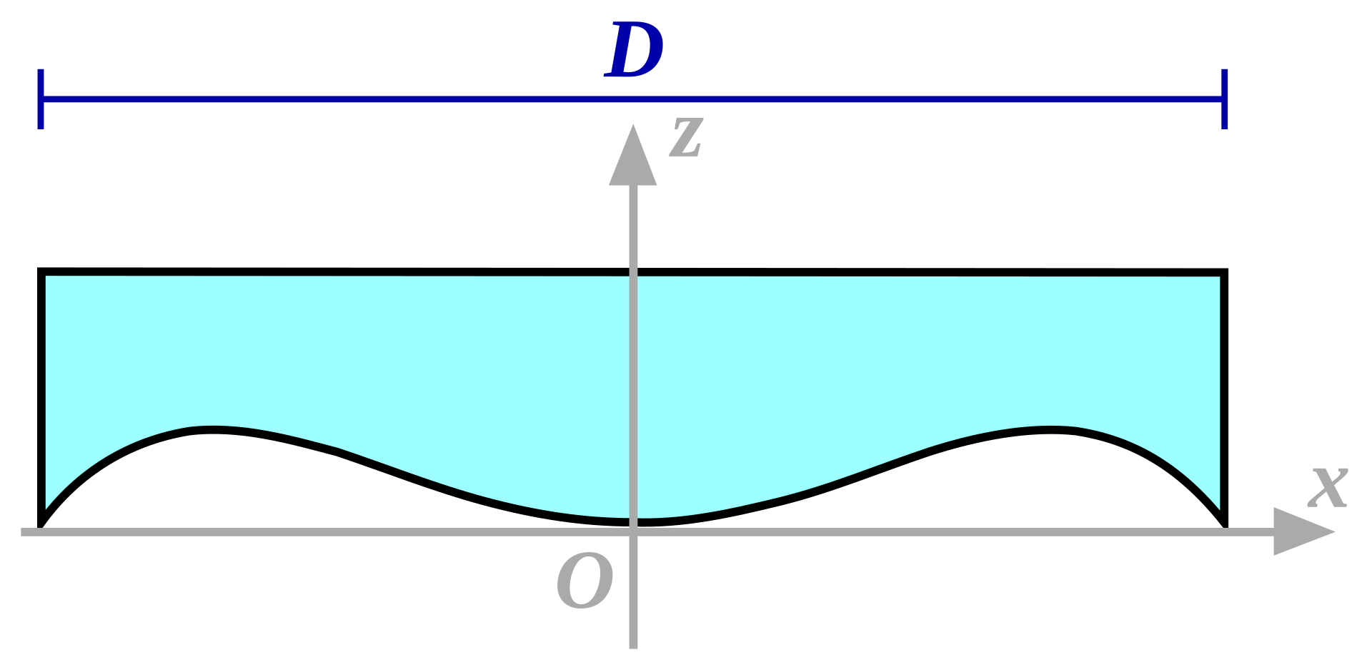
Fig 5: SFRplus target for Imatest – it’s height is 783 mm between the horizontal black bars, which means, that the reproduction ratio on film is 33:1 – source: fotosaurier/Imatest – original information graphics from IMATEST
Over years I did – like many other amateur-photographers – compare real-world photos of analog vs. digital processing. But I was never satisfied, because this method gave me only subjective impressions – it did not create reproducible figures, to generate a precise description of the results!
I collected intensive experience with IMATEST on more than 150 lenses over meanwhile 5-6 years using the digital pictures generated by digital sensors (4,9 to 102 Megapixels) of seven different DIGICAMS. During this time, my Standard Digicam to compare lenses was (and still is) Sony A7R4 (62 Megapixels) – since it had arrived in the market (2018/19).
IMATEST (Studio) software delivers MTF-based resolution data – as it can do that separately in three RGB-channels, it also delivers lateral CA-data. Using the Target structure of Fig. 5, the software selects 46 local areas, and runs the MTF-measurement automatically for all these 46 areas. The following picture demonstrates the automatic areas, which are typically selected – but you could choose others as well:
Fig. 6: The 46 magenta rectangles (called „ROI„) frame the Edges in the target, at which the 46 MTF-measurements are made – source: fotosaurier/Imatest
These are the curves, which are generated from each digital picture (black&white):
Fig. 7: Summary of the IMATEST-results for the OM28mm f/2.8 at open aperture f/2.8 on Sony 62 MP-sensor (A7R4) – explanation see text beneath – source: fotosaurier
The upper left curve shows the edge-profile at center of the target (ROI no. 1, which is the left (vertical) edge of the center square in Fig. 6). From this graph the edge-rise between 10% and 90% is taken from the x-coordinate in pixels. The lower left curve is the MTF-curve (contrast over spatial frequency) for the same location. From this graph the MTF30 value (Frequency at 30% contrast) is taken: follow the horizontal line at 0,3 MTF-value to its section with the curve and take the frequency on the abscissa. The right curve shows the MTF30-values of ALL 46 ROIs plotted over the distance from the center in the 35mm-fframe.
I have resumed the IMATEST test-method in more detail in this article here in my blog!
B. Digital measurement of resolution on analog film
Now I decided to make the following experiment:
Take a photograph of the IMATEST-target on analog film;
digitize the picture with a film-scanner;
analyse the resulting digital picture with IMATEST.
For the tests, which I describe here, I used the following hardware:
Fig. 8: Analog SLR Olympus OM-4 Ti with Zuiko Auto-W 28mm f/2.8, loaded with „fresh“ Agfa APX100
Camera for the shooting on analog-film: Olympus OM-4Ti
Film: B&W negative film AgfaPhoto APX100, iso125, developed in Rodinal 1+25 (8′)
Scanner: reflecta RPS 10M film scanner
The OM-4Ti (about 25 years old) and the lens (nearly 50 years old) work still perfect. I let the OM-4Ti automatically generate the exposure time: from 0.4 seconds to 1/250 seconds. The densitiy of the negatives was pretty constant on the film-strip! I use a sturdy tripod, which is made for use with long astronomical telescopes.
With this method I hope to use the full analyzing-power of IMATEST-software on a picture-frame, which is generated through the lens WITHOUT the typical artefacts, which digital sensors MAY generate in the optical path of a historical lens.
ON THE FILM we have now the IMATEST target-pattern, which allows to make a fast and powerfull analysis of optical data over the full picture frame – also very close to the edges and into the corners. This pattern is superimposed by the typical grain-structure of the light sensitive layer – and potential light-diffusion-effects within the film thickness. Both (analog) effects LIMIT the resolution, which can be achieved on FILM.
My first and major interest was always focused on the observation of the enormous difference between the center-resolution (see Fig. 7), which is digitally measured on A7R4 with ca. 3,000 LP/PH or higher) and corner-resolutions of <200 to 600 LP/PH on the sensor .
The question is: are the low values on edges and in coners of the frame, measured with the digital sensors, an artefact, caused by the different light-path? We know definitely about these effects with rangefinder-lenses, which have a very short back-distance between last lens and film, causing big trouble on sensors of mirrorless cameras. This is today well known, to be mainly caused by the thick filter-stacks in front of the sensors (creating field-curvature and cromatic aberrations with analog lenses).
It has been shown, that this can partly be „cured“ – or at least reduced – by reducing or deleting the filter-stack, and/or putting a positive lens (so-called „PCX-filter“) in front of the lens-sensor-combination.
The 35mm-negative-film:
I made my first attempts to photograph the IMATEST-target on film with
b&w-film Agfa APX100, iso 100
which is still available as „fresh“ product. For this first step I decided to stay with b&w-film, because I can process it myself under controlled conditions. With colour negative film I would have an external influence, which I could not control! Just for resolution this means no restriction in the information, because CA-errors also blurr the B&W-picture!
I did the devellopment of the b&w-film myself with Rodinal.
The A/D-converting:
The negatives were digitized through my film-scanner reflecta RPS 10M,which offers a maximum linear resolution of 10,000 pixel per inch (PPI).
To me, this step seemed to be very important: to avoid new artefacts from the digitizing algorithm. So I chose a spatial frequency, which is higher than the expected limiting spatial frequency of the film: I set the scanner at 5,000 ppi. On pixel-level this corresponds to an imaging-sensor of ca. 33.7 MP (for 24mm x 36mm).
From my earlier estimations I had found, that a normal recording film for general imaging purposes should correspond to a digital FullFormat-sensor with 20-12 MP.
The picture height, which the scanner digitally delivers (24mm minus a bit of crop to frame the target safely), was 4,676 pixels and so the „Nyquist Frequency“ of the scanner set-up corresponds to 2,338 LP/PH – corresponding to an effective sensor-size of 32,7 Mpxls.
Fig. 7 shows the b&w-picture, which was generated with the scanner:
Fig. 7: Scanner-output from the b&w negative-film Agfa APX100 from Olympus OM 28mm f/2.8 at full aperture f/2.8. Picture-hight of this original scan is 4.676 Pxls. You see, that the light-fall-off of this lens into the corners is very moderate … and the linear distortion with exactly 1% acceptable as well! – source: fotosaurier
Let’s have a closer look into the structure of this image – in Fig. 7a you get an impression of the grain structure of the films emulsion at about 200% enlargement of the 33 MP-image:
Fig. 7a: Overview of the grain-structure at ca. 200% enlagement of original scan in Fig. 7. The pixel-size here is 5,3 µm – the grains of the film are bigger than the pixels – source: fotosaurier
Following picture is the MTF-curve of the analog image „as scanned“ (in the center of frame):
Fig 8: MTF-curve in. Center (ROI no.1) of OM-Zuiko 28mm f/2.8 at f/2.8 – source: fotosaurier
The „noise“ in the curve is caused by the film-grain, which is about the same size as pixels.
Fig. 9: Here we look at about 1,000% into the pixel-structure of the scanned image. At the edges of the dark rectangle (where the resolution is analysed!) the grain-diameter is about the same size. Only some local „grain-clusters“ are considerably bigger – source: fotosaurier
Previous trials had shown, that with a film with this grain-structure, this digital image-size would give adequate results for MTF and resolution.
In the case of a digital sensor of a digicam I avoided generally to use RAW-data, which would have urged me to use my own very personal „development-parameters“ in Lightroom or other software to generate the final picture. I use OOC-JPEG-Data at „Standard“-settings, due to generate conditions (all important parameters set to „zero“), which are transparent and reproducible for everybody with the same camera-model! That means: it would also have been possible to create pictures with much higher resolution results in Imatest, e.g. by setting higher sharpening-parameters or the „clear“-mode.
Now with a film-scanner I had to go myself through a very intensive process of defining the „development-parameters“ in Silverfast. Starting with the setting to 5.000 ppi for the basic scan-resolution. With 10.000 ppi, which is offered with this model, you will get no REAL increase in EFFECTIVE resolution.
However, using the „Multiple Scan Mode“, you extend the accessible resolutions above the „Nyquist Frequency“, which would be 2.383 LP/PH, corresponding to a Picture size of 32,7 MP.
My target was, to reach about the same level of resolution in the center of the scanned images on analog film as with the Sony A7R4 images, which means in the range of 3.168 LP/PH, which is the Nyquist Frequency of the Sony Sensor.
This corresponds with a resolution of 260 Lines/mm.
I came close to this with the following settings:
Fig. 10: Scan-parameters in Silverfast 8 on film-scanner RPS 10M – source: fotosaurier
See the complete results here:
Fig. 11: Analog on film resolution results of Olympus OM 28mm f/2.8 SLR-lens with b+w-film APX100, scanned with RPS 10M film-scanner – source: fotosaurier
The interpretation of this in comparison with the measurement-results on the 62 MP-sensor of the Sony A7R4 (Fif. 2) has been given in the first section of the Article.
Finally I asked myself, whether a PCX-filter (lens) could improve the resolution-artefacts which are found on the sensor? But I found no real positive effect.
Fig. 12: Resolution of OM 28mm f/2.8 lens with PCX-3m lens on the Sony A7R4-sensor: no improvement at all – source fotosaurierFig. 13: Soon I will enter a new article, showing the performance of this wideangle-lens on seven different cameras – link not yet available … stay tuned!
Fig 1: From left to right – Topcor R 30cm f/2.8, Arsat Yashma 300mm f/2.8, Tamron SP LD (IF) 300mm f/2.8, Minolta AF Apo-Tele 300mm f/2.8, Canon EF 300mm f/2.8 L IS USM
Attention: I part from my „crazy lenses“ due to my age: it takes too much time to take care for my optical baybies! If you are interested in the Topcor R 30cm f/2.8, please look at https://www.ebay.de/itm/146462870630 or leave a price-proposal in the comment-section (this is seen only by me) or by mail to webmaster@fotosaurier.de
1. On my time-machine:
I own the Topcor R 30cm f/2.8, which I am looking at here, since a few years – but I have not used it too often. It is very heavy, long and dark, giving the impression of a tank-breaking weapon: you definitely will get trouble at any security check nowadays … and in the best case you will earn compassion instead of admiration! Too bad, because it is an ingenious piece of optical engineering.
Information about Topcor lenses today are rare and not always reliable. I will restrict myself to reliable information and I will try to verify legends … or destroy them.
So I entered my time machine and travelled back into the year 1958. I was 13 years old at my arrival there – and at the Topcon (Tokyo Kogaku) factory I met a team of innovative engineers, who were fanatically burning for the QUALITY of their products – and really proud of it! The year before (1957) they had introduced a new SLR-camera (Topcon R), which was designed in Bauhaus-style, i.e. with clear and modern lines – and they were ready to ignit a firework of innovations around the SLR-concept within the next few years (from first-in-industry TTL-exposure-metering to first electric winder).
And they had introduced a line of lenses for this SLR-system-camera, among which the Topcor 30cm f/2.8 peaked out. Another „first-in-industry“-innovation.
I looked around in the photo-stores and could not find any Canon- or Nikon-SLRs there: the dealers told me, that both companies were just bringing out SLRs. It seemed, that the Topcon-people had considered the German SLRs, which were already on the market, as their competition. Personally at that time I was already a SLR-user (of my father’s Contaflex – which means, that from time to time my father was still allowed to use it himself).
Everybody, who is acqainted with the rules of the market, would have expected, that shortly after an innovation like the Topcor R 30cm f/2.8, the major competitors would bring out a similar product.
But that did not happen – so I returned in my time-machine. Finally I found out, that it took the new japanese competitors more than a decade! And there was no comparable Lens in Europe, as far as I could see. 13 years later Nikon presented a prototype, to be tested during the Olympic Winter Games of Sapporo in 1972.
The real next step was taken by Canon with a 300mm f/2.8 Lens for their new FD-System, using a lens made of FLUORITE in 1973 (some say 75)! This was finally 16 years after the arrival of the Topcor-lens … and just in that year, when Topcon stopped the production of their supertele-lens.
2. The known facts:
This Topcor R 30cm f/2.8 monster-tele-lens with 300mm focal length was presented to the world in 1958 („Topcon Club“ says 1957!) – one year before Canon or Nikon started to produce any SLR – and 13-16 years before any other lens- or camera-maker presented such a fast 300mm tele-lens. Not only at the 1964 Olympic Games in Tokyo but all the time until 1972 it was without any competition. As a consequence, there even was produced quite a number of lenses with Nikon mounts! Next to Topcon, Canon brought out its Canon FD 300mm f/2.8 S.S.C. Fluorite lens in 1973 – setting the level for professional superlele-lenses for the next decades and until today. Just a few years later Topcon went completly out of the business with SLR-cameras and lenses. Sad, but even the extensive book „Topcon Story“ by Marco Antonetto and Claudio Russo (1) does not answer the question „why?“. Today Topcon is a market-leader in geodesic instruments.
Stephen Gandy (3) estimates – cameraquest.com – that 700-800 lenses have been produced in total during 18 years of production.
Fig. 2a: R.Topcor 1:2.8 f=300mm on Topcon SuperD- source: fotosaurier
The lens is made of six single lenses in four groups – of which lens no. 6 (group 4) is the filter (diameter 39mm), which is, of course, part of the optical design! This filter is an early (maybe the first) example of a filter which is positioned in a slot in the rear part of the lens-body. In the book „Topcon Story“ (page 128) there is an error in the spreadsheet listing of the data of the R.Topcor-lenses: the data in the last line are the data of the „300mm 2.8“ and not of the f/5.6-lens. Here the no. of elements is „five“, which is correct, when you don’t count the filter as an active optical member …
The lens has a preset diaphragm and has a built-in sunshade (telescoping in two stages!). It is 383 mm long (from camera-flange to front-edge of the pulled-back sunshade – total length with shade pulled out is 477 mm) and weighs 3.1 kgs (without front and rear caps). Measured at my sample (ser. no. 34.1359). The initial sales-price was $ 1.125,–. (In the literature you will find: 415/412 mm length and 3.3 kgs weight).
It may be interesting to mention here, that right away from the introduction of the first Topcon-SLR, an extremely ambitious lens-program was planned – however, realized only partly. The Topcor R 13,5 cm f/2.0 (6 lenses) had also preset diaphragm and it was discontinued with the Topcon RE camera system – so it is said to be extremely rare. It has a yellowish color cast (due to rare-earth-glass?), not a big problem with todays digital cameras …
However, a 50mm f/0.7 lens, which is mentioned in „Topcon Club“ only, was never made for the SLR-camera market – maybe, this was one of the very early oscilloscope-registration-lenses, which are also known from Germany and GB even at WWII-times.
And a 1000mm f/7 catadioptric lens was only experimentally made in 1958.
„Topcon Club“ (2) writes about this:
„The interchangeable lenses which appeared with the appearance of TOPCON R are various kinds of the Auto Topcor of 35mm/100mm, and R TOPCOR (a preset diaphragm) of 90mm/135mm/200mm/300mm among these – although the bright thing and the dark thing were prepared about 135mm and 300mm – it should mention especially – it is the „high-speed lens“ of 135mm f2 and 300mm f2.8. 50mm f0.7 – such a bright lens was already completed during wartime by the Tokyo optics. Do you believe it ? Although possibly this grade was an easy thing, even so, the 300mm f2.8 lens will be an astonishment thing in 1957. I talked in detail on „the page of TOPCOR“ about this lens. We have to wait for marketing of the product of NIKON which is the next 300mm f2.8 lens at any rate till 1977. However, TOPCON did not build the super telephoto lens 500mm /800mm those days. Furthermore, the Refrector Topcor 1000mm f7 is appearing in the catalog in ’59. However, this was not launched regretfully.“
Later – from 1969 on – a RE Topcor 500mm f/5.6 telephoto-lens was even produced with automatic diaphragm and meter coupling!
Can such a fast long telephoto lens like this early 300mm f/2.8-design without Fluorite- or ED-lenses be any good – on the scale of professional photography? There are hints, that rare-earth glasses were used to make these lenses (also for the other famous 13,5cm f/2.0, also supplied since 1958). But I do not know details about this.
I will answer the question about the optical quality here – also comparing this lens with a modern top-notch tele-lenses like Canon EF 300mm f/2.8 L IS USM, which I personally classify as today’s state-of-the-art reference, supported by photo-friend Thomas, who borrowed his Canon lens to me.
Finally I will take a glance on a state-of-the-art modern astronomical refractor, which normally does perform at diffraction-limited resolution on stars!
Topcor 30cm f/2.8 – The Optical Performance on analog film (year 1969):
Stephen Gandy (3) wrote in his blog:
WIDE OPEN its resolution was 56lines/mm center and 34lines/mm at the edges. By f/8 it was 80 lines/mm center and 65 at the edges. Many normal lenses don’t achieve this sharpness — much less 300/2.8 leviathans ! Camera 35 summed it up by saying „INCREDIBLY FANTASTIC.“ I would have to agree. „
(In the original text in Stephen’s blog, the reported resolution values are noted as „56mm“ or „34mm“. I have taken the freedom, to correct this to what it should read: lines per mm, „lines/mm“!)
The resolution values, which I use in my digital IMATEST measurements, typically are given in „Line-pairs per picture-height“ = „LP/PH“. Picture-height being 24mm with 24×36-format, you have to divide the „lines/mm“-values by two to get to „line-pairs“ – and then multiply with 24 to achieve LP/PH.
The highest given value of 80 lines/mm corresponds to 960 LP/PH stopped down to f/8 in the center or 760 LP/PH at f/8 at the edge – the lowest value 34 lines/mm with open diaphragm at the edge corresponds to 408 LP/PH.
What does that mean?
In 1969 the test results for resolution were measured on film – „Modern Photography“ used Plus-X Pan with standardized development – and the reading of the „just resolved“ line-pattern was done with a standardized enlarging glass … I personally used the method myself at that time, too, and it is quite reproducible as long as the same person does the reading … It is somewhat sensitive to the vision-capabilities of the reading person! And of course the grain of the analog film material (negative b&w film!) is the limiting factor for the resolution-reading on film for really high resolutions.
Today’s modern 24 MP-sensors deliver resolutions of 2,000-2,400 LP/PH using MTF30 (30% contrast) as the parameter for reading out the resolution values from the MTF-curve. My Sony A7R4-Camera (62 MP), which I use for my measurements, has a Nyquist frequency of 3.168 LP/PH and delivers up to 3.800 LP/PH-readings with the best known lenses.
The following spreadsheet gives an overview on the physical data of the Topcor-lens and the other lens-monsters, analysed here:
Fig. 3: Physical Data of the five 300mm f/3.8-Lenses – source: measured by fotosaurier
3. Topcor 30cm f/2.8 – Optical Performance
My IMATEST-Results of the optical properties of the Topcor R 30cm f/2.8 lens:
To exclude potential vibration-initiated degradation of resolution in my test-shots at these long focal-lengths I used my heavy (>10 kgs) and sturdy astronomical telescope-mount:
Fig. 4: My massive astronomical lens mount – here with SonyA7R4 attached to Topcor 30cm f/2.8 – source: fotosaurier
Fig. 5: The set-up keeps the lens and camera steady even at 0,4 seconds. – source: fotosaurier
Following you see the results of my IMATEST-measurements:
Fig. 6: Optical measurment-results for Topcor R 300mm f/2.8 adapted to Sony A7R4 with 62 MP – resolution values given in LP/PH – source: fotosaurier
Fig. 7: Resolution measurement-results for Topcor R 300mm f/2.8 as graph – source: fotosaurier
The lens is unique at that time regarding to „speed“ – an extremely ambitious piece of optical engineering. Remind, that the distortion is practically zero and the CA-area in the center 0,8-1,4 pixel – 1 pixel at Sony A7R4 is 3,8 microns on the sensor!
What is center, what is part way and what is corner? In the following graphs from IMATEST you see: „Part-Way“ is the large part of the picture extending close to the narrow side (left/right). „Corner“ is the narrow area outside the second dotted circle on the picture below.
Fig. 8: „Center“ resolution is calculated as mean from the values inside the inner circle (in my setting always two values), „part way“ is the mean of all values between the inner and outer circle, „corner“ is the mean of all values positioned outside the outer circle – source: fotosaurier
Fig. 9: Topcor R 30cm f/2.8 resolution plotted over radius of picture circle – source: fotosaurier
So, let’s compare the measurements to the value, that were given in analog times on film:
The comparison in the spreadsheet Fig. 10 shows: The lens „out-resolves“ normal analog films by far! Stopped down it reaches the limits of the analog medium even at the edges of the frame!
Fig.10: „Camera35’s“ resolution measurements for Topcor R 30cm f(2.8 of 1969 on film compared with digital IMATEST values (at 30% MTF = „MTF30) with Sony A7R4 – source: fotosaurier
I found no real technical explanation, how Topcon-engineers managed to generate this phantastic lens at that time without ED/LD/AD/Fluorite-glass. There is a second tele-lens – the 13,5cm f/2.0, also introduced 1958, with first-in-industry potential – and finally the Topcor 2,5cm f/3.5 super-wide, which surprises with best-in-class resolution values (see my blog-article on historical 24/25mm-lenses!).
If somebody knows the secret: please, tell us!
Look at a sample picture taken with the Topcor at the end of this article at 65% enlargement size (see Fig. 24).
Now, let’s have a glance on some other historical Superteles:
Fig. 11: From left to right: Topcor R 300mm f/2.8, Canon EF 300mm f/2.8 IS USM, Minolta AF Apo-Tele 400mm f/2.8, Tamron SP (60B) 300mm f/2.8 LD (IF), Arsat Yashma-4H MC 300mm f/2.8
4.The Reference: Canon EF 300mm f/2.8 IS USM
Fig. 12: Canon EF 300mm f/2.8 IS USM – source: fotosaurier
Canon EF 300mm f/2.8 IS USM is rated as the reference of this class of lenses. In this case it is not the latest „Mk II“-version of it, which came out 2011 – but the first version of 1999, which is tested here. It represents nevertheless already the top-class of the super-teles (as all its predecessors since 1973!)
Here are the IMATEST results of its optical properties:
Fig.13: Optical properties of Canon EF 300mm f/2.8 IS USM from my IMATEST-measurements, with autofocus – source: fotosaurier
And here the Graphs of resolutions center, part way and corner:
Fig. 14: IMATEST-Resolution (LP/PH) of Canon EF 300mm f/2.8 IS USM – center – part way and corners – source: fotosaurier
Not may comments necessary to this – the figures and graphs should speak for itself … Just to mention: the distortion at the Topcor-lens is even lower than that of the Canon – but both are neglectable for a supertele!
Canons leadership in this class of professional supertele-lenses was generated by the policy, not to drop a product into the market, which was „just possible“ at present, but to persue a consequent plan for the future: to solve the „secondary spectrum“-problem of long tele-lenses, which means to use extreme „anormal dispersion“ lens-materials, which do the job without optical compromising.
So in 1975 – 2 years after Nikons first presentation of its first 300mm f/2.8 ED-lens (which was not very convincing and had to be replaced four years later by the ED-IF-version) – Canon introduced their FD 300mm f/2.8 Fluorite-Supertele, in which they used a front-lens made of fluorite-monocrystal material (no glass!) and a UD-glass-lens. This lens was already praised close to perfect (absence of chromatic aberrrations). Canon accepted for this a compromise, which made the lens longer and heavier: to protect the soft and sensitive fluorite-crystal-material in the front lens, there was a fixed additional plane protection element of glass in front!
Finally new fluorite-glass-formulations became available, which allowed to drop the sensitive crystal-lens. Over the introduction of Autofocus (EOS – 1987) and still more glass-elements, Canon finally introduced the legenday lens EF 300mm f/2.8L IS USM in 1999 with very fast AF and image-stabiliser, which is tested here.
Enjoy the results!
5. Finally – three more 300mm f/2.8-teles:
Minolta AF APO-Tele 300mm f/2.8 (1985)
Tamron SP LD (IF) 300mm f/2.8 (60H) (1984)
ARSAT MC Yashma-4H 300mm f/2.8 (1990?)
For these three lenses I also have to thank foto-friend Thomas, who borrowed them to me!
5a. Minolta AF APO-Tele 300mm f/2.8 (1985)
Fig. 15: Minolta AF APO-Tele 300mm f/2.8 – source: fotosaurier
This lens had a mechanical defect: the diaphragm could not be closed below f/5,6. However: in these lenses principally mainly the open aperture is really significant – why should you carry around such a weight, to make pictures with f/11?
Fig. 16: Optical properties of Minolta AF 300mm f/2.8 Apo – source: fotosaurier
Fig. 17: IMATEST-Resolution (LP/PH) of Minolta AF 300mm f/2.8 Apo – center – part way and corners – source: fotosaurier
This Minolta lens comes closer to the Canon-legend than any of the others – but with quite some distance in resolution in the corners open aperture.
This is the shortest and lightest lens of the quintuple, which arrived even one year before the Minolta – containing two low-dispersion (LD) lenses – with manual focusing:
I do not know much about this lens. Funny about it is to me, that in most cases, when it is offered as a used lens, it is given the addendum „sovjet lens„! In 1990, when it was delivered first (I saw other sources with the date 2007 …) the Sovjet Union no longer existed – which means that, ARSAT being located in KIEW, the lens has UKRAINIAN roots.
As far as I know, it was generally produced in Nikon-mount.
Fig. 22: Optical performance of Arsat MC Yashma-4H 300mm f/2.8 – source: fotosaurier
Fig. 23: Resolution graphs of ARSAT MC Yashma 300mm f/2.8 – source: fotosaurier
Open aperture and stopped down the lens is convincing in the center – about 10-15% below the other superteles – but with still very good CA in the center.
From f/4.0 it is also very good in the large part of the frame – just 10% below the Topcor.
In the corners it is on par with the Topcor open aperture – but it does not improve so much while stopping down. For analog film use it was also a good lens – with exception of the softer corners with typical CA-values of non-apochromatic lenses … and a much higher distortion than all the other superteles.
What about apochromatic correction in supertele-lenses?
Lenses of 300mm f/2.8 need apochromatic correction to be really sharp. The chromatic aberrations („secondary spectrum“) are the major restictions in sharpnes for these long focal lengths all over the frame! All these lenses, tested in this report, have apochromatic correction – in varying degrees of perfection! In the ARSAT Yashma the apo-correction is only partly successful.
Herbert Börger
fotosaurier, Berlin 13.02.2023
Literature:
1- „Topcon Story – Topcon Enigma“ by Marco Antonetto and Claudio Russo, by Nassa Watch Gallery, Collectors Camera Publishing, CH 6907 Lugano, Switzerland – 1997
This, the first super fast long telephoto lens produced for any camera system world wide, came to the market in 1957. This was a large and heavy lens, with a 130mm maximum diameter, a length of 412 mm and a weight of 3.3 kg. The optical design was one of 6 elements in 4 groups. The selling price, at the time, was 135,000 Yen making it the most expensive lens on the market. Special filters slide into a slot at the rear of the lens barrel and this lens was probably the first to use this method. Unlike the 135mm f2 R Topcor, this lens was listed in catalogues into the later half of the 1970s. Because of it’s large aperture it was chosen as the official lens of record for the Tokyo Olympics. An odd thing concerning this lens is that many of those remaining have been modified for the Nikon mount, while those with the original Topcon mount are very scarce. The early lens case was made of leather but later on Topcon began supplying a hard case with the TOPCON emblem promontory displayed. The R Topcor 300mm f2.8 lens still compares favorable, with regards to regards to sharpness and contrast, to modern lenses with fluorite elements. Today this lens is almost forgotten but was highly praised in former times.
3- Web site of Steven Gandy: „https://www.cameraquest.com/top30028.htm“
Fig. 24: Mathäuskirche in Hambühl, seen from 1,2 km distance with Topcor 300f2,8 (taken at f/5,6 with Sony A7R2 at iso800) – narrow vertical crop of nearly full frame, which you see here at about 65% enlargement – „ooc“ – no post-treatment of the picture) – source: fotosaurier
A few weeks ago I was blessed, having an Angénieux 50mm f/0,95-lensand a „Biotar 50mm f/1.4″, at the same time in the same place !
An Angénieux 50mm f/0,95-lens in perfect optical quality and with aperture-mechanism and rehoused into a perfect Sony-E-body, focusing to infinity and ready for measurement in my optical IMATEST-Lab…. this is really a „unicorn“!
Fig. 1: Ultra-rare 50mm f/0.95-lens for Cine 35 movie-format – this lens-series (10mm, 25mm and 50mm) founded Pierre Angénieux‘ high reputation in cinematic optics! – source: fotosaurier
The „Biotar 50mm f/1.4″, in great overall condition, which I even did no know about, before I saw it for the first time.
Fig. 2: One of the best high-speed-lenses ever made in Jena – Biotar 50mm f/1.4 of 1955/56 for Pentaxflex AK-16 cine-camera system – professional performance for professional use! – source: fotosaurier
Photo-friend and co-nerd Thomas handed out both ultra-rare lenses to me for closer optical inspection. I am a happy man!
Fig. 3: Two very rare lenses at the same time in the same place … in my IMATEST-Lab! Sheer happiness! – Source: fotosaurier
Angénieux 50mm f/0,95 (Type M1):
Thomas has proven, that it is possible to re-house the Angénieux-lens for general photographic use with infinity focus:
Fig. 4: The early super-fast Angénieux 50mm f/0.95 lens 0f 1954/55 here in a „Unikat„-version – the basic lens is directly fitted to E-Mount for Sony – source: fotosaurier
Starting in 1953 Pierre Angénieux brought out a series of lenses with f/0.95. In 1953 it was firstly the 25mm f/0.95 (which became the most famous Angénieux lens due to the use in NASA-spaceflights to the moon!) made for cine 16mm format and the 10mm f/0.95 for 8mm-cine.
A few months later he pushed out also a version for 35mm-cine: the 50mm f/0.95 – probably this was in in 1954 – originally in C-Mount. Hartmut Thiele dates this to 1955. It is important to understand, that this is not a lens made for still-photogray amateur use – but Pierre Angénieux showed here all his knowledge dedicated for professional cine-use. He went to the limits of everything, which was possible with glass-types and design- and production-methods at that time!
If you need more information on Pierre Angénieux, please look up my Blog article here!
Following my measurements on the IMATEST-target the picture-circle, that this lens covers is 37mm – so it is falling a bit short from the 43mm needed for covering the still-photo-35mm-full-format (24 x 36 mm).
Fig. 5: Picture of IMATEST-Target through Angénieux 50mm f/0.95 at f/0.95 in the 24 x 36 mm full-frame of the Sony A7R4 – Source: fotosaurier
This test-set-up generates the following resolution-measurement results:
Fig. 6: Resolution at center/part way/corner of Angénieux 50mm f/0.95 on Sony A7R4 (60,2 MP-sensor – 9.504 x 6.336 pixels!) at standard distance full-frame (24×36) – Source: fotosaurier
In spite of the heavy darkening in the corners, the system does still generate results, but these readings are not very reproducible … these corner-readings are located clearly outside the picture-circle for this lens!
So I made a second set-up with the camera set a little bit further away from the target, so that the individual measuring areas move somewhat towards the center of the picture and do not suffer too much from the dark areas out of the picture circle of the lens.
Fig. 7:Angénieux 50mm f/0.95 moved a bit backwards from the target – measurement-areas (marked magenta rectangles) moved somewhat further towards the picture center – avoiding overlap with the dark corners – this picture is at f/8, showing a sharper limit to the dark corner-areas! – source: fotosaurier
Now the furthest measurement locations are at 82% of the full-frame picture radius, clearly inside the bright circle which this lens covers at 86% of full-frame radius!
The result is seen in the following picture:
Fig. 8: Resolution with refocussed Angénieux lens 50mm f/0.95. The corner-resolution-values are still located outside the Cine35-picture-frame!!! The „peak“ at f/4 in the corner reading is real – no error – never seen anything like this with any other lens! – source: fotosaurier.
In Chapter 4 at the end of the article I will ad thwe measuremts at cine-format for all three lenses (Super 35: 18,66mm x 24,89mm). This will give more realistic resolution-readings. The Super35 crop-mode on the A7R4 is 6.240 x 4.160 pixels.
2. Carl Zeiss Jena Biotar 50mm f/1.4:
About the same time, DDR-based Carl Zeiss Jena created a high-speed lens for its own Pentaxflex AK-16 cine-camera system in Pentaflex-16 mount.
It seemed logical to follow the already successfull BIOTAR-formula and it came out around 1955 or 1956 the Biotar 50mm f/1.4:
Looked at with the sensor of the Sony A7R4, the picture-circle is a bit larger than with the Angénieux … there are only minimal dark corners!
Fig. 10: Full-frame picture of IMATEST-target through Biotar 50mm f/1.4 at f/1.4 – Source: fotosaurier
Of course, we have here the same situation, that the corner-measurements are quite a bit outside the cine-picture frame of typically 16mm x 22mm:
Fig. 11: Biotar 50mm f/1.4 in the same frame as Angénieux seen in Fig. 7 – source: fotosaurier
I will also with this lens repeat the measurement, restricting the resolution-target to the cine-picture frame – see section 4 at the end of the article.
The results show for both lenses, that the resolution in the center is extremely high – even wide-open! Both lenses are extraordinary lenses of their time – the mid-1950s!!!
Unique: „first-in-industry“ point of view for the Angénieux 50mm f/0.95 in its extreme speed, without sacrifycing to the center resolution!
3. Canon Lens 50mm f/0.95 for rangefinder (Canon7) cameras with LTM 39mm – of 1969
As we are just talking about early historical high-speed lenses, the step to the famous CANON 50mm f/0.95 (for rangefinder) is logical. It is a step of 15 years in time – and this time the lens is really dedicated to 35mm still-photo full-format 24mm x 36mm!
Fig. 12: Angénieux 50mm f/0,95 of 1954, left, and Canon 50mm f/0.95 of 1969 / the normal still-photo-version here – Source: fotosaurier
Here is my comparable resolution-measurement with two samples of (s.n.18924 and s.n.22372) of the Canon 50mm f/0.95 on Sony A7R4 for this lens at full 24×36-format:
Fig. 13: Resolution-Graph of Canon 50mm f/0.95 on Sony A7R4 (60,2 MP) – Source: fotosaurier
Fig. 13a: Resolution-Graph of Canon 50mm f/0.95 on Sony A7R4 (60,2 MP) – Source: fotosaurier
To allow for the necessary rangefinder-coupling besides the huge rear lens, this lens is „cut free“ at the edge for this purpose.
Fig. 14: Cut-away at the 50f/0.95 Canon’s rear lens, to allow for the rangefinder-coupling! – source: fotosaurier
However, the 50mm f/0.95 lens was also released in a version for video cameras, with an additional engravure „TV“ on the nameplate: consequently these lenses were delivered with C-mount. As these lenses do not need the rangefinder-coupling, the rear lens is not cut at the edge here:
Thank you, foto-friend Thomas, for the 50mm f/0.95 TV-lens rear section photo.
4. Finally: Resolution-Data of these Lenses, measured for the Cine Super35-format, which the Angénieux and CZJ Biotar Lenses are originally dedicated to – on all three lenses:
a) Angénieux 50mm f/0.95 – at Super35-format:
Fig. 16: Angénieux 50mm f/0.95 at Super35-frame on Sony A7R4 – absolutely phantastic for this „first-in-speed“ – source: fotosaurier
b) Biotar 50mm f/1.4 – at Super35-format:
Fig. 17: CZJBiotar 50mm f/1.4 at Super35-frame on Sony A7R4 – absolutely phantastic at one stop slower – source: fotosaurier
c) Canon 50mm f/0.95 – at Super35-format on Sony A7R4:
Fig. 18: Canon Rangefinder 50mm f/0.95 – primarily dedicated to still-photo 24×36 but also delivered as a TV-version – just a bit better than the Angenieux, but 15 years later! – source: fotosaurier
All three lenses have very low chromatic aberrations in the center but the Canon peaks out in maximum CA, Biotar and Canon are close to zero in distortion, while the Angenieux has around -1% distortion, which is still excellent for such an early, extreme lens!
5. Appendix:
Here you see all properties of the three lenses in detail – for 24×36 (full frame) and Super 35 (cine-format).
What was the real improvement in SLR-wideangle-lenses since the invention of the retrofocus principle over the last 65 years? Does my personal judgement from analog-film-days which lead to the definition of „legendary optics“ – which I kept in my lens-portefolio over that time – correlate with objective resolution-measurements? Here are my findings.
Actualisation: Im my first published version there was an error regarding the year of appearance of the Topcor 2,5cm-lens, which was communicated to me by a reader: thank you: it’s 1965 instead of 1959! But this difference does not change anything in my findings and conclusions …
1 – Introduction
24mm focal length is a real milestone in spreading the field of the view in wideangle lenses, coming down from FL 35mm over 28mm. For the SLR-camera-user this age started with the appearance of the retrofocus lenses in the 1950s. Several designers came out with this optical principle within three years – with Pierre Angénieux earning the honours of being FIRST (in time and quality – 1950, 35mm f/2.5) in this disciplin.
This is a report about SLR-lenses for 35mm-still-foto-cameras with focal lengths (FL) between 23mm and 25mm.
This is a report about a number of legendary lenses, which I happen to own or could lend from a friend („phothograf“), most of them being milestones of optical engineering in their respective design-periods.
Fig 1: three of the very first historical retrofocus-lenses with FL 24mm and 25mm – source: fotosaurier
Over the decades of my own practical use of SLR-lenses (of nearly all makers-brands!) has lead me to an understanding of the quality for normal photographic use.
This collection of test candidates does NOT claim to be a COMPLETE collection of all design legends of 24mm/25mm. There is a large gap in time with prime-lenses between 1984 and 2015. That means: the legendary first historical aspherical lenses in this range are missing in the comparison. If I ever will be able to get hold of them for a test, I would update this article. The modern lenses tested for comparison are (of course) all aspherical types!
In spite of the fact, that important legendary lenses of the 1980s and 90s are missing here, this report allows to draw some interesting conclusions about important steps in optical lens-engineering, which finally lead to Ultra-Wideangel-Lenses which have uniform resolution and contrast over the complete field of view (FoV).
I have always looked for a method to show the quantitative progress in optical quality of photographic lenses over the nearly last 100 years – and I think I have found a good way to understand this progress with my new comparison-charts (Fig. 4 and Fig. 5 see below). What was surprising: the progress over time is independent of the lens-maker and brand. It is generated by a sequence of milestone-like innovations by singular design-legends, innovative calculation progress, creation of new glass-formulations and finally the lens-making-process – espacially allowing for the production of aspherical lens-surfaces! Once the innovation-step is basically made, it is spreading around the globe very quickly (typically within one or two years!).
There are few lenses, which stand out of the general quality-development curve, reaching a higher level of resolution earlier than most others – to be seen here mostly in Fig. 5:
ATTENTION: These measurements are made with USED lenses today, some of which are more than 60 years old! There are influences from ageing and wear (even abuse …) which have become part of the lens-properties when we measure them after long time. However, I only make measurements with samples of lenses, if the optics are clear and undamaged and the mechanics do not show excessive wear or abuse.
Fig. 2: Starting with big-big negative front-meniscus-lenses (at left Angenieux Retrofocus 24mm f/3.5 and Zeiss Jena Flektogon 25mm f/4) the lens-designers soon learnt to reduce the front-lens diameter (at right: Distagon 25mm f/2.8 for Contarex and Olympus OM 24mm f/2,0), creating better results and generating lens-bodies, which were more acceptable – source: fotosaurier2 – Data section for 15 historical 24/25mm-prime lenses, 3 modern 23/25mm prime lenses and 4 modern zooms at 24mm-setting:Fig. 3: optical measurement results of all measured lenses – source: fotosaurier
Out of this Chart I have filtered two separate charts, showing the development of RESOLUTION over the decades.
Fig. 4 shows the center-resolutionopen aperture (blue) and stopped down to the aperture with the highest resolution (green) in the center:
The second chart is showing the corner-resolution at open aperture (blue) vs. the best resolution-value stopped down (green) in the corners (mean value over all four corners) – where „corner“ means a value of 88% – 92% of the full picture circle of the lens which is 21.5 mm radius:
Fig. 5: Corner Resolution-values of 21 Lenses at FL 23-25mm at open aperture (blue) and optimum aperture (green, which means: the aperture at which the weighted mean of all the 46 measurement-places over the 24x36mm-frame is maximum. (The maximum corner resulution-value of the individual lens may be higher.) – source: fotosaurier
You see, that nearly all of the difference in resolution of historical top-notch wideangle-lenses for SLR is in the corners of the picture (and of course also continuously in-between center to corner areas). This is easy to understand, because the difficulties for lens-correction rise dramatically with the FoV, which is here 84 degrees corner to corner diagonally.
Besides the resolution, there are other important properties, which improved dramatically over these six decades of lens-engineering history:
a – Chromatic aberration (CA in pixel): It is very low in all these lenses in the center. It typically ranged between 4 and 8 pixels in the corners for the very first lenses of this type. It stayed around 2-3 over the time before aspherical lens-surfaces could practically erase it. Today with the best modern lenses, the value is close to zero (under 0.5) without camera correction and zero with correction.
Among the early lenses the Zeiss Distagon 25mm f/2.8 (though not really outstanding in resolution compared to the other early lenses) pops out, because it had already values of 2-2.5 pixel in the corners – together with the „unicorn“ Topcor 2,5cm f/3.5.
Please consider, that the CA-value in pixel for the same lens is the higher the smaller the pixel size of the sensor is – here 1 pixel is 3.77 µm.
b – Linear distortion (%): distortion shows – from the beginning – the biggest differences between the legendary lenses of the different designers and brands. The designer has to do a compromise-job in each lens, balancing out the design between resolution, chromatic aberrations and distortions. 0,5 pixel is a very good CA-value even acceptable for acrchitectural work (though „zero“ would be better, of course), 0,75-1,0 pixel is a good compromise-value and 1.5 pixel just acceptable for alround use.
Looking at the spread-sheet Fig. 3, it is surprising, that Angénieux with the very first retrofocus-lens of this wide angle decided to go for nearly „ZERO“ distortion in his design! He had gone close to zero in the 35mm and 28mm-designs before that, too! Probably he wanted to give a statement of his art, because this was really difficult at that time … At the same time he accepted a somewhat higher CA of 7-8 pixels (corresponding to 0.03-0.04 mm). In my collection of top-notch lenses such a low distortion does not appear again before the modern Zeiss Batis Distagon 25mm f/2.0 – and only the legendary 1971 Minolta MD 24mm f/2.8 (including the VFC-Version) came very close with ca. 0.18-0.29% distortion in my measurements.
c – The close-focusing system: there are further innovations to consider, e.g. the lens-design for close focusing. Here one of the important innovations is the floating-element close focusing system – introduced 1971 by Nikon and Minolta first for wideangle lenses as far as I know. This is one of the early merits of the two 1971/75 24mm-Minolta-lenses.
3 – Conclusions:3.1 Center-resolution:
Since the early days of geometrical optic lens-design with Petzval, Abbe and Seidel, lenses could be designed absolutely perfect for nearly unlimited image-quality (resolution and CA) „on-axis“, which means: in the center of the picture-field … And the famous designers did it all the time – as soon as they used 4 or more elements in a photographic lens-system.
The first time, I found a proof for that, was with my resolution-measurements on Bertele’s first Ernostar 100mm f/2.0 from 1923 (a four-element-design WITHOUT COATING!). Compared to the legendary Leitz Apo-Macro-Elmarit 100mm f/2.8 from 1987, this lens achieved 98% of the resolution in the center – but only in the center! See my Ernostar-Bog-Article here. (This was the very first report in my photo-blog …)
So, it is not really surprising, what Fig. 4 is telling us: all top-notch lenses show a very high resolution level in the image center since the invention of the retrofocus wideangle design in the 1950s – and they are all on the about same level – though being historical lenses with up to 65 years of age on their back! The reason for that result is, of couse, that only legendary lenses of all brands are taken into the comparison! Maybe the Takumar-lens happens to be one of the weaker examples …
The Olympus OM 24mm f/3.5 „shift“ drops down somewhat against its neighbours. That is no quality issue: this lens has an image-circle diameter of 57mm for up to 10 mm shift! It came out 1984 long before Canon brought out its famous tilt-shift-lenses … Look at the corner-resolution result of this lens in Fig. 5 – it resolves extremely even over its FoV!
in this graph I marked two horizontal lines: one for the resolution of 2.000 LP/PH (linepairs per picture height), corresponding to the resolution of a 24 MP-sensor, which today is the de-facto-standard for modern digicams. It normally has 4.000 by 6.000 pixels – and 4.000 pixels in the picture height, corresponding to 2.000 Linepairs. At the same time it is just (+15%) not mucht below the 32 MP which I estimate for the resolution of modern analogue (general purpose) film emulsions.
The other (upper) horizontal line marks the 3.184 LP/PH Nyquist-frequency of the Sensor in the Sony A7R4-digicam. This is physically the limiting resolution-value for the camera itself. Today, however, the software-algorithms in the camaras can generate structures in the picture, which are typically 15 – 20% higher in resolution, compared to the Nyquist-frequency. And they do this without creating an artificially looking „oversharpened“ picture! Good job!
This means: All the legendary historical 24/25mm-retrofocus-lenses for SLR-cameras do out-resolve the modern 24 MP-Digicams in the center – mostly even with open aperture! And many of these lenses even come very close to (or exceed) the Nyquist-Frequency of my 60,2 MP digital camera.
Among the historical lenses two examples peek out a little bit (they peek out much more in the graph for the corner-resolution!):
The legendary 1965 Topcor 2,5cm f/3.5 exceeds the Nyquist-frequency of 3.184 LP/PH – and stopped down to f11 it is in the center the highest resolving of my 24/25mm-lenses until today. Together with the tremendous result of its corner-resolution it is one of the exceptional lenses, which I call my „UNICORNS„. Until today, I have not found any explanation for the astonishing early level of performance of this lens – how could that have been achieved? (15 years before the next-best Olympus-lens!) – and who did it? – and where did this person go afterwards, when Topcons innovative power faded out, to bring in her/his inginuity? (… to Olympus?). (This observation refers to other early Topcor-lenses al well!)
The other unicorn peeking out here is the Olympus OM 24 mm f/2.0 of 1973. In my lens-collection it is exceeded only by the 40 years younger Zeiss Batis 25mm f/2.0. But, to be honest, the difference is not really that dramatical – considering the four decades …
Referring to the zoom-lenses (set at FL 24mm) in this test: I just was curious, where the modern zooms would stand in such a comparison. We learn that the 1kg-Monster-Tokina 24-70mm zoom at 24mm has one of the best results – even at f/2.8 … in the center of the picture.
At the end of the line-up of 21 lenses I put the Fujinon-Zoom 32-64mm f/4 at 32 mm on the Fujifilm GFX100 (33x44mm – 102 MP), which corresponds to FL 26mm on „full-frame 35mm“. This shows, that for an essentially higher resolution in the picture-center, we today have to go to a larger sensor-format.
3.2 Corner-resolution:Fig. 5 contains the important informations of this comparison-test. It shows, that step by step all the improvements in innovative design, glass-formulations and aspherical surface-generation were needed to bring finally the corner-resolution of the picture up on par with the center resolution at 24mm focal length, which is possible today – but only with the use of aspherical lens-elements!
In the graph for the corner-resolution I have added a third horizontal line, which marks the resolution at 50 Lines/mm – corresponding to 600 LP/PH. This is needed to judge the corner-resolution of the early historical lenses.
In the 1960s a wideangle-lens was rated „very good“, when it achieved a resolution of 40 Lines/mm (Modern Photography and others). I have written an article about this already here (in German). Open aperture most super-wideangle-lense started open aperture in the range of 26 to 32 L/mm in the 1950s and 60s. Stopped down practically all the tested historical lenses surpassed the 40 L/mm-limit.
From 1958 on (ENNA) the stop-down corner-resolution rises continualy (with the exception of the two „unicorns“, already identified in Fig.4) until end of the 1970s, it arrives close to the 2.000 LP/PH-level, which means: from now on the top-notch-lenses out-perform standard analogue fine-grain film (1977 Nikkor and 1984 Olympus). This last step was then achieved by the use of extraordinary dispersion glass-types.
The two „unicorns“ in this test arrive much earlier at this level: the Topcor 2,5cm f/3.5 out-performs analogue film already in 1959 and the 1973 Olympus OM 24mm f/2.0 exceeds this and comes close to todays modern aspherical lenses.
The modern aspherical prime-lenses are represented in my test by two very different samples:
There is the 23mm f/4 Fujinon, which originally is a GFX-lens – but in this test it is measured in the 24x36mm-Mode also with 60.2 MP on the GFX100, achieving the state of the art for 24x36mm lenses (Batis and Sigma-i) as a middle-format lens!
Just as I made my measurements for this test, the SIGMA i-Series 24mm f/3.5 arrived as a representative of a new thinking: no „impressive“ technical data – but (hopefully) impressive preformance instead. The result shows: it achieves reference status on a 60.2 MP-sensor with corner-resolution at 85-95% of center-resolution, plus zero-distortion, zero-CA and very close focussing!
Also great news: modern zooms like the Sigma G 12-24mm f/4 – measured at 24mm – arrive now at this level of prime-lenses also in the corners!
As I had no samples of the early historical aspherical lenses in this test, we can not see, in which steps the aspherical lens surfaces moved the wideangle-performance in the picture-corners to the present level.
Maybe this gap can be filled out in some future times.
NOTE 1 – All resolution-values, which are published in this article, refer to MTF30 – what means: the point on the MTF-curve (see Fig. 7), which hits the 30% contrast value.
NOTE 2 – in Part II of this Article I will share some more informations about each individual lens (including pictures, MTF-curves and lens-schemes).
Appendix: Method of measurement and definition of results
I use the set-up and software by IMATEST with the original IMATEST-Target. I use the large SFRplus-Setup-Image with a physical hight of 783mm bar-to-bar vertically. The distance from target to lens-flange is 0,97 meters. In this area 46 targets are analysed and I share MFT30-weighted-mean-resolution-values (all-over, center and corner), edge-sharpness, linear distortion and maximum lateral CA-values.
Resolution-values are given in Line-Pairs per Picture Height (LP/PH) – where the picture-height is always 24mm. Edge-sharpness is given in pixels (width 3,77 µm).
For the measurement I used a SONY A7Rm4 with 60,2 MP-resolution which has a pixel-width of 3,77 µm. The theoretical resolution-limit of the sensor is 3.184 LP/PH (Nyquist Frequency).
The camera setting is used basic as delivered from factory at ISO100 and exposure-compensation of -0.7 stops, using out-of-camera JPEGs. All measurements are made with the identical camera-body (which is important for a precise comparison: I have used one other (earlier) body of this model in comparison, which gave resolution-values between 50 and 200 LP/PH lower than my own camera-body). The repeatability with this method I estimate at 2-2.5%, using ALWAYS manual focusing on the lens with maximum focusing enlargement (11.9-fold) in the camera-viewing-system. Measurement is repeated with re-focusing until a stable maximum resolution at open-aperture of the lens is found and then pictures of the resolution-target are taken with the focussing made wide open for all full down-stops of each lens.
Edge profile (edge-sharpness) is the width of the rise from 10% to 90% intensity at a dark-bright edge in the test target – measured in pixel (width 3,77 with the camera used) – Example shown here for the latest 24mm-prime-lens SIGMA i-Series 24mm f/3,5 – at open aperture f/3,5:
Fig. 7: Edge-profile (top) and MTF-curve (bottom) from the IMATEST software – here the perfect graphs for the brand new Sigma 24mm f/3.5 – at open aperture. I will publish these Curves for all the lenses in PART II of this article – source: fotosaurierCromatic Aberration (lateral in the picture-plane) is also measured in pixel separate for red against green and blue against green over the full picture field – in the spread-sheet I note the maximum value, which is in most cases for blue and for most historical lenses in the corners of the picture – sometimes however in the intermediate area.
For more details of testing read my special blog-Article here.
Copyright: Herbert Börger
Berlin, March/April 2021
Would you expect, that the optical performance of your photographic lenses can be seriously influenced by the operating temperature? Have you ever realized lack of sharpness in extreme environmental temperature conditions?
The simple answer is, of course, that within the specifications for use, given by the makers, there should be no such concern. But it is not that simple.
For amateur astronomers with their mostly very long telescope-focal-length optics (mirror or lens) this fact is very common:
before using the instrument in the clear and mostly cold winter-nights, you have to put the telescope early enough outside (shielded against due) to bring it into a thermal equilibrium with the ambient air at the time you start your observations. The reason: during essential temperature-changes of the optical components (mirrors, lenses) and their mounting devices, their surface-shapes and adjustment change and destroy the extremly precise optical alignment – until the thermal equilibrium is restored. The refractor-lenses may be mounted to allow for some thermal differences, but large mirrors have to be mounted and adjusted extremely precise, so that the cooling-down of the mount, that holds the mirror, may even generate mechanical tension on the mirror – and that generates optical distortions! So we should remind: the absolute temperatures are not the problem – but the thermal transition stages from warm to cold or opposite way!
This fact is also an important design aspect for telescopes: the preferred structure is „as open as possible“ to allow the air to circulate and to generate a good heat-exchange with the internal telescope structure to speed up this process. While the air gets colder during the night, the instrument’s optics can follow close enough to keep the temperature difference low.
There is an impressive document in the archives of the Mt. Wilson Observatory (near L.A., USA) describing the „first-light“-moment of the new 2,5 meter mirror telescope (Hooker-Telescope) on November 1, 1917 – use this link to the adventurous story! („First light“ is the moment, when somebody looks through the finished instrument for the first time.) Here the first-light moment at Mt. Wilson is described near the end of the long text in this link and shows, what a three hour cool-down time made to the optical properties of the 2.5 meter mirror, (which was made by George Willis Ritchey – and allowed for the detection of the expansion of the Universe by Edwin Hubble shortly after taking this telescope into service.).
Picture 1: 2,5 m (100 inch) Hooker-telescope on Mt. Wilson: just struts hold the mirrors to ease the circulation of air for for a fast achievement of temperature equilibrium – source: Ken Spencer, CC BY-SA 3.0 <https://creativecommons.org/licenses/by-sa/3.0>, via Wikimedia Commons
Many instruments in astronomy are closed assemblies, using a corrector-plate (Schmidt-system) or meniscus-lens (Maksutov-System) in the entry of the tube and the mirror at the rear-end (catadioptric telescope – see also my specific blog-article here.) The big disadvantage of these closed systems is the „inertia“ in cooling down due to the closed volume in the telescope tube. Therefore often slits around correctors and mirrors are placed, which allow for sufficient circulation of air through the tube – and even active ventilation is used to shorten the period to reach equilibrium. In some big modern telescopes, the mirror may even be actively temperature-controlled.
Picture 2: „Closed“-tube optical system Maksutov-Cassegrain-Teleskop – source: Wikipedia – Author: Halfblue – http://creativecommons.org/licenses/by-sa/3.0/.
Long telephoto-lenses for normal photography can not be open systems, because the lens-barrels definitely have to be tightly sealed to avoid the invasion of dust, humidity or corrosive gases.
This means, that you have to plan and prepare carefully to bring your equipment to ambient temperatueres in time to avoid these thermal problems. For photographic equipment this would equally refer to the situation, when you come from climate-controlled environment (e.g. hotels) into wery hot (and humid) areas. There is an additional problem, that in bringing cold equipment into hot-humid environment, there might be condensation of humidity on the lenses/mirrors.
This problem is even more delicate with catadioptric lenses (mirror/lens-systems often called just „mirror-lenses“ – in German „Spiegel-Objektive“). In these the surface-shape of the mirrors and the adjustment from mirror to mirror is extremely sensitive for the optical performance of the lens-systems.
I have to-date not realized this with focal lengths of up to 350 mm (though it might be also there to a certain dergree) – but this is definitely an important aspect for focal lengths between 500 mm and 1,000 mm or longer.
From which focal length on these problems may occur, will mainly depend of the type of optical system – and of course the resolution of your cameras sensor!
Here I want to show you this effect with an example of a catadioptric lens of 800 mm focal length: the Vivitar Series 1 Solid Catadioptric 800mm f/11, used on the Sony A7Rm4 (60,3 MP, 35mm format – 3.77 µm pixel-pitch).
It was the first day this year with just sligtly above zero outside temperature (+2 degree Celsius) and very clear air. At ca. 1:15 p.m.I set out the 800mm f/11 lens on the tripod on the balcony and tried to focus on my favorite landscape test target: a roof-top at about 40 m distance.
The advantage of this target is, that it has large AND fine details, low contrast AND high contrast areas and – most important – a sufficient depth, so that I can detect focusing errors very well!
Picture 4: Overview picture – complete field of view of the „roof-top“ landscape target in ca. 40 m distance taken with Sony A7Rm4 and Vivitar Series 1 Solid Cat 800mm f/11 – this is the „sharp“ picture after the cool-down period of the lens – source: fotosaurier
It was nearly impossible to meet the positive focus position – so I did the best guess and made the photo – and here is the 100%-crop around the focus-position, which is the first steel spring at the right side of the roof edge:
Picture 5: The 67% detail of the focus-area (clamp and spiral-spring!) made 15 minutes after setting the lens outside. Best guess of focus, however, you will find no sharper point in front or behind – the distance scale on the lens says 50 meters in this non-equilibrium temperature situation – source: fotosaurier
At this point of time the lens internally is still on room temperature of about 21 degrees … starting to cool down for about 15 minutes, which it took me to set everything up and focus carefully – but desperately, becaus no really sharp focus was seen in high viewing-magnification.
I had focused using the maximum viewfinder enlagement in the Sony camera and was sure: this is not a really sharp picture. But I could not find a better focus. Picture 5 is a 67% crop of the image taken. And as the subject has some depth: no – there is no better focus to be seen on this picture in front or behind the plane of the spring.
I left the lens with camera in this position for three hours and refocused the lens: now I experienced a quite snappy focus – and you can see the same crop-area here:
Picture 6: The 67% detail of the focus-area (refocused!) after additional 3 hours of the lens outside – source: fotosaurier
The gain in sharpness is damatical – and it exists over the whole field of view, not only in the plane of focus! Also out-of-focus areas show higher contrast now.
However, it connot be ignored, that this catadioptric lens in this picture does by far not use the potential 3,168 Line-Pairs per Picture Height Nyquist frequency of the cameras sensor. My estimate is, that we have here an MTF30 of about 1,100-1,200 LP/PH. So either the three hours of cool-down time were not yet sufficient – or the lens may be not better than this.
(The 1,200 LP/PH MTF30-resolution would correspond to 100 Lines/mm in older „analog“ data. Very good CATs in the 1970s had center-resolutions (measured on film) between 50 and 60 Lines/mm. This relation makes sense, as the difference (factor 0.6 lower for film!) may be owed to the effect of grain and the thickness of the emulsion.)
The „Solid Cat“ 800mm f/11 is a massiv piece of optics – the lens barrel is nearly completely filled with glass, as you see in the lens-scheme:
Picture 7: Lens-scheme of the Vivitar Series1 Solid Cat – source: Perkin Elmer Patent application
It is an absolutly unusual mass of glass – so I would not exclude, that the cooling time should even be longer to reach the thermal equilibrium. My plan is, to make a sequence of photos taken in shorter intervals and over a longer time – as soon as the outside temperatures go down again.
I am not so happy with the fact, that I had to use landscape-scene-shots to demonstrate the performance of the lens, however, for 800mm focal length my IMATEST testing-arena is too short. Maybe I will make a parallel IMATEST-trial then with a 500mm CAT.
So, please, consider this as a first teaser for the topic which has shown clearly, that photographic lens performance may seriously suffer during the time, a lens is undergoing strong temperature-change and before equilibrium is reached.
I promise to come back with a more elaborate research-plan soon.
Herbert Börger
Berlin, December 4th, 2020
Aphorism of the day: Scientific research is most successfull, when it brings up more new questions than it has answered. (fotosaurier)
Aktueller Hinweis in eigener Sache: Ich verkaufe die meisten meiner CAT-Objektive – die Links zu Ebay finden Sie folgend. / A personal hint: I sell most of my CAT-lenses now – find the links to Ebay following.
Die Erkenntnisse aus Teil II führen zu dem Schluß, dass für die ab den 1950er Jahren aufkommenden katadioptrischen Foto-Objektive aus den vielfältigen, bereits für Astro-Anwendungen bekannten „katadioptrischen Dialyten“ (Brachymediale) abgeleitet wurden, von denen einige schon bis zu 150 Jahre bekannt waren und unter denen Maksutov eine spezielle Variante ist.
Eine kurze Geschichte der Katadioptrischen Foto-Objektive:
Mit dem starken Aufkommen der Spiegel-Linsen-Objektive in den 1960-70er Jahren bildeten sich spezielle Konstruktionsmerkmale heraus, die in dieser Form bei astronomischen Fernrohren meist nicht zu finden sind:
a) Außer der Tatsache, dass die Foto-Optiken sehr robust und hermetisch dicht gebaut sind, wurde zunehmend auf die Bohrung im Primärspiegel verzichtet! Das bedeutet, dass die Strahlen, die vom Sekundär-Spiegel zurück geworfen werden, nicht mehr durch eine Öffnung im Hauptspiegel zur Kamera bzw. Filmebene gelangen, sondern durch einen unverspiegelten zentralen Bereich der Spiegelfläche durch das Glas des Spiegelkörpers treten.
Das bedeutet, dass der Innenbereich der Optik zwischen den beiden Spiegeln noch besser hermetisch abgeschlossen ist. Es bedeutet gleichzeitig, dass der zentrale Bereich des Spiegelkörpers auch noch als brechendes Linsenelement im Strahlengang einbezogen ist. Dieser Bereich bildet dann oft zusammen mit 1-3 weiteren Linsen den Sub-Apertur-Korrektor im Strahlengang nach dem Sekundärspiegel. Er muss aus Linsen-Glas allerhöchster Güte bestehen, da dieser Bereich des Hauptspiegels – im Falle eines Mangin-Spiegels – dreimal von jedem Lichtstrahl durchlaufen wird!
b) Immer häufiger treten nach 1965 Mangin-Spiegel auf, was ja der Grundkonfiguration des Hamilton-Teleskopes entspricht. Zuerst finden sich Primärspiegel als Mangin-Typ, bald auch beim Sekundärspiegel bzw. in beiden Positionen gleichzeitig oder auch nur beim Sekundärspiegel. Wie wir oben gesehen haben (Hamilton-Teleskop) ist der Mangin-Spiegel bereits ein Grund-Element des kadadioptrischen Dialyts – für sich genommen ist er meines Wissens nie als Teleskop oder Astrokamera verwendet worden.
Bild 1: Mangin-Spiegel – Quelle: Wikipedia – Autor: not known – https://creativecommons.org/licenses/by-sa/3.0/
Neben der Wirkung als Element der optischen Rechnung liefert der Mangin-Spiegel zwei weitere Vorteile für das Foto-Objektiv:
Die an der polierten Glasfläche anliegende reflektierende Spiegeloberfläche ist in der Mikro-Oberflächenstruktur wesentlich glatter als eine aufgedampfte Aluminium-Schicht auf ihrer „offenen“ Seite, die auch noch mit einer transparenten Schutzschicht (meistens Si02) überzogen werden muss.
Die Verspiegelungs-Schicht ist gegen den Zutritt von korrosiven Gasen, Feuchtigkeit etc. perfekt geschützt und behält langfristig seine uneingeschränkte Wirkung. Dies alleine wäre schon ein ausreicheder Grund, um diese Bauweise zu bevorzugen!
c) Foto-Objektive katadioptrischer Bauart benötigen zur Abschirmung gegen Falschlicht rohrförmige Blenden um den Zentralen Strahlen-Durchlass im Zentrum des Primärspiegels (nach vorne in Richtung des Sekundärspiegels) bzw. um den Sekundärspiegel herum (in Richtung Hauptspiegel), um die Kamera vor einfallendem Falschlicht zu wchützen. Auf dem folgenden Linsenschnitt sind die Tubus-Blenden und das Problem des Falschlichtes gut zu erkennen:
Bild 2: Linsenschnitt mit Abschirmtubus-Blenden gegen „Falschlicht“am Olympus Zuiko Reflex 500mm f/8 (in diesem Bild ist der Lichteintritt rechts!) – Quelle: Olympus Produktbeschreibungs- und Spezifikationsdatenblatt zum Objektiv
An diesem Bild kann man gut erkennen, dass ohne diese beiden Blenden Lichtstrahlen durch die ringförmige Apertur-Öffnung (rechts) direkt und ohne Reflexion an den Spiegeln auf das Zentrum des Hauptspielgels und damit auch in die Kamera gelangen könnten! Eine Gegenlichtblende vor dem Objektiv kann das nur dann sicher verhindern, wenn die Gegenlichtblende extrem lang wäre – was natürlich dem Objektiv-Konzept widerspricht …
Die Existenz dieser rohrförmigen Blenden im zentralen Bereich hat Auswirkungen auf die sog. Obstruktion – also die Abschattung der Lichtstrahlen im Zentrum der Apertur:
Bei Strahlenbündeln, die vom Bildfeldrand schräg in die Optik einfallen, werfen die Tubusblenden einen Schatten auf den Hauptspiegel. In der Folge ist nicht mehr die gesamte Ringförmige Spiegelfläche „aktiv“. Sie ist in der Breite des Blendentubus unterbrochen. Man kann das bei geeigneter Bildstruktur an den außerfokalen Apertur-Ringbildern von Lichtreflexen sehen, wie folgend in dem absichtlich unscharf gestellten Aufnahme des Hausdaches gut zu erkennen ist:
Bild 3: „Tubusblenden-Schatten“ bei den außerfokalen Unschärferingen im Randbereich mit dem Olympus OM Zuiko Reflex 500mm f/8: unten-links und -rechts sieht man die kleinen „Packman-Ringe“ – die Öffnung weist zum Bildzentrum hin. – Quelle: fotosaurier
d) Die große Korrektor-Linse in der Lichteintritts-Apertur dient immer auch gleichzeitig als Tragstruktur für den Sekundärspiegel. Wie im Teil I ausführlich beschrieben wurde, führt die „Obstruktion“ durch den Sekundärspiegel im Strahlengang zu einer Kontrastverringerung des Beugungsbildes 1. Ordnung. Aber wenigstens werden durch das Fehlen von Tragspinnen die dadurch verursachten Beugungs-Spikes in den Bildern einer Punktlichtquelle vermieden, wie sie beim normalen Newton und Cassegrain auftreten.
Vorbemerkung: die Einordnung bestimmter Objektive als „Meilenstein“, die ich hier vornehme, ist rein SUBJEKTIV und basiert auf meinem – begrenzten – Wissen bzw. meiner Erfahrung. Mir ist bewusst, dass andere Fotografen und Beobachter zu etwas anderen Schlüssen kommen können, die ihrer eigenen Erfahrung entsprechen.
An dieser Stelle möchte ich noch einmal ins Gedächtnis rufen, dass in den 1950er bis 70er Jahren gegenüber „langen“ Teleobjektiven (>200mm Brennweite) nicht nur Kompaktheit (Baulänge) und geringes Gewicht für die „CATs“ sprach, sondern vor allem die Freiheit von Farbfehlern (Chromatische Aberration, „CA“) – im Verhältnis zum Preis! Es gab zwar in den 1970ern bereits die ersten farbreinen Telekanonen mit Fluorid-Linsen – aber zu einem extrem hohen Preis unter Verwendung eines sehr empfindlichen Materials. Den Preis konnten/wollten sich sicher wenige Amateurfotografen leisten. So bin ich überzeugt, dass die „Blüte“ der katadioptrischen Teleobjektive hauptsächlich vom Amateur-Segment getragen war.
Darüber, warum die katadioptrische Objektivbauform fast völlig wieder verschwunden ist, werde ich am Ende dieses Artikels einige (begründete) Vermutungen anstellen.
Hier nun mein kurzer Überblick auf die Zeitskala und die Entstehungsgeschichte geschlossener katadioptrischer Systeme, die als Foto-Objektive geeignet waren oder spezifisch dafür gebaut wurden.
Ich führe hier auch die mir bekannte Grundlagenentwicklungen ebenfalls im Zeitstrahl mit auf, damit die zeitliche Dimension mit einem Blick sichtbar wird.
Ich führe dann Foto-Objektive auf, die aus meiner Sicht Meilensteine der Entwicklung solcher Optiken darstellen. Dies ist keine vollständige Beschreibung dieses Objektiv-Segmentes! Ich versuche derzeit Informationen über alle jemals gelieferten Photo-CATs zu sammeln und hoffe in einigen Monaten eine fast vollständige Liste veröffentlichen zu können.
Fast alle bekannten katadioptrischen Teleobjektive wurden für das Kleinbildformat gerechnet. Einige wenige zeichneten Mittelformat 6×6 oder 6×7 aus: Carl Zeiss Jena Spiegelobjektive 500mm und 1.000mm, Kilfitt 500mm und 1.000mm und Pentax 6×7 1.000mm f8 – soweit mir bekannt ist.
1814 –
Grundlagen-Erfindung (Astronomie) des Katadioptrischen Dialyts (auch „Brachymedial“ genannt) durch Hamilton und darauf folgend eine große Reihe von Varianten und Weiterentwicklungen.
Bis in jüngerer Zeit hat eine italienische Firma tatsächlich noch Hamilton-Teleskope/-Kameras für astronomische Zwecke geliefert (Ceravolo).
1930 –
Grundlagen-Erfindung (Astronomie) der Schmidt-Korrektor-Platte – daraus entstanden Schmidt-Kamera und Schmidt-Cassegrain-Teleskop
1940/41 –
Grundlagen-Erfindung (Astronomie) des Maksutov-Korrektor-Meniskuslinse – daraus entstanden das Maksutov-Cassegrain-Teleskop – genau betrachtet ist es aber eine Sonderform des katadioptrischen Dialyts.
ab 1945 –
Maksutov-Cassegrain 3,5″ f/12-Teleskope – Lieferung großer Stückzahl des Teleskops an sowjetische Schulen, gebaut (anfangs) vermutlich in Nowosibirsk. Wenn Sie wissen wollen, wie das Schul-Teleskop aussah, folgen sie bitte diesem Link zu einer sehr kompakten Biografie Maksutovs auf Prabook. Dort sehen Sie ein Bild von D. Maksutov mit „seinem“ Schul-Teleskop vor ihm auf dem Schreibtisch. Mit ähnlicher Spezifikation wurde es in Polen als „PZO“ hergestellt und in der DDR von Zeiss als „Telementor„. Diese Geräte wurden auch (da sie Devisen brachten!) in den Westen verkauft.
Bemerkenswert ist, dass die Motivation, ein extrem robustes und haltbares sowie wartungsarmes Fernrohr für Schulen zu schaffen, bei Dimitri Maksutov zu der ursprünglichen Idee für das Meniskus-Tesleskop-Design führte. Ich sehe darin ein Beispiel, dass auch das Streben nach Gemeinwohl zu hervorragenden Innovationen führen kann!
QUESTAR Maksutov-Cassegrain-Teleskop 3,5″ (in Großserie gefertigt bis heute)
Klassisches Maksutov-Cassegrain, Brennweite 1280mm f/14.4 (Spezifikation ab 1961) – wurde und wird auch als Teleskop-Tubus („Field-Model“ oder „Birder“) mit Okular- oder Kameraanschluss geliefert.
Ein Kult-Klassiker der Amateur-Astronomie. Aber auch die NASA soll einige beschafft haben …
Bild 4: Questar-3,5″-Teleskop mit ausgezogener Taukappe – Quelle Wikipedia, Autor:Hmaag – https://creativecommons.org/licenses/by-sa/3.0
ab 1936 bis in die 1960er Jahre
wurden mindestens in Deutschland (Zeiss), Japan (Nikon) und Russland (GOI) und USA (Kodak) große semi-transportable (meist katadioptrische) Spiegelobjektive für militärische und satellitengestützte Anwendungen entwickelt. Diese waren ausschließlich vom Maksutov-Typ und hatten Brennweiten von 1.800mm – 8.200mm. Viele Informationen dazu gibt es im Übersichtsartikel von Marco Cavina in diesem Link. Auf diese umfangreichen Erfahrungen konnten sich die Optik-Unternehmen dann nach dem 2. Weltkrieg bei der Entwicklung von katadioptrischen Wechselobjektiven für Spiegelreflex-Kameras stützen.
vor 1958 –
Erste Maksutov-Cassegrain-Teleobjektive für SLR von LZSO, Sowjetunion: MTO 1.000mm f/10.5 und MTO 500mm f8 – erhielten eine Goldmedallie auf der EXPO in Brüssel 1958.
Ich weiß nicht, wann genau diese Maksutov-Cassegrain auf den Foto-Markt gebracht wurden. Es muss noch unter der strengen Überwachung von Dimitri Maksutov selbst gewesen sein, der ja bis 1964 lebte. Gibt es Leser, die da weiter helfen können?
Bild 5a: MTO-500mm f/8 – Quelle: fotosaurier
Bild 5b: MTO-1.000mm f/10 – Quelle: fotosaurier
Das archaische Design und die solide Bauweise führten dazu, dass die Optiken (bis heute) von Fotoamateuren liebevoll als „Russentonnen“ bezeichnet werden. Herstellerbezeichnungen waren und sind MTO, Arsenal, Rubinar. Nicht immer waren die Optiken leider in der Qualität konstant, was oft an verspannt eingebauten Spiegeln gelegen haben soll. Ein Bericht dazu (Dr. Wolfgang Strickling) finden Sie hier.
1959/1961 – Nikon bringt nach den russischen MTOs bereits 1959 sein erstes CAT mit ehrgeizigen Daten auf den Markt, das Reflex-Nikkor 1.000mm f/6.3 – und bereits 1961 folgt ein Reflex-Nikkor 500mm f/5. Ab den frühen 1970er bis in die 2000er Jahre bietet dann Nikon kontinuierlich das „Reflex-Nikkor-Trio“ 500 f/8 + 1.000 f/11 . 2.000 f/11 an. Viele Details findet man in dem Artikel von Marco Cavina – für die Liebhaber der italienischen Sprache! Die 2.000mm f11 wurden demnach alle von 1971 bis 1975 in zwei Versionen gefertigt. Das eklärt wohl zur Genüge, warum Ihnen das 2.000er CAT so selten in „freier Wildbahn“ begegnet.
Bild 6: Reflex-Nikkor C 500mm f/8 – Quelle: fotosaurier
1961 – Carl Zeiss Jena
stellt das katadioptrische „Spiegelobjektiv“ 500mm f4,0 auf der Leipziger Messe vor (Entwickelt ab 1955 von Dr. Harry Zöllner, W. Dannenberg. (Kurze Zeit später kommt auch ein Spiegelobjektiv 1.000mm f5,6, die sog. „Stasi-Kanone“, hinzu). Die Optiken sind für Mittelformat 6 x 6 gerechnet und geliefert worden!
Frei zugängliche Darstellungen von Linsenschnitt, Auflösung und MTF-Kurven stehen mir bisher zu diesen Optiken nicht zur Verfügung. Allerdings gibt es einen fabelhaften synoptischen Artikel von Marco Cavina, in dem das Jena-Spiegelobjektiv 500mm f/4.0 und das Mirotar f/4.5 im Detail ausführlich beschrieben und verglichen werden.
Bereits 1941 hatten bei Zeiss die Konstrukteure Robert Richter und Hermann Slevogt ein CAT-System (Richter-Slevogt-Teleskop) entwickelt und angemeldet, das dem kurz vorher in GB angemeldeten „Houghton-Teleskop“ (s. Teil II) ähnelt. Wahrscheinlich wussten beide Gruppen damals im Krieg nichts voneinander.
Auf diese Entwicklungen von 1941 geht offensichtlich dieses Carl Zeiss Jena-Spiegelobjektiv zurück.
Cavina äußert in seinem Artikel die Vermutung, dass die optische Leistung des Jena-Objektivs nicht an das folgend beschriebene, kurz danach heraus gekommene Objektiv von Zeiss Oberkochen heran kommt, da es vermutlich als IR-Fernobjektiv für Aufnahmen auf IR-Schwarzweißfilm entwickelt wurde.
In dem Blog „Zeissmania“ (Teil II) finden sich einige Aufnahmen,die der Autor selbst mit dem Zeiss Jena 1.000 f/5.6 gemacht hat (Website der Burgenländischen Amateurastronomen BAA).
1963 – Zeiss Oberkochen (West)
stellt das MIROTAR 500mm f/4,5 vor und fertigt 200 Exemplare für Contarex. Zeiss-Konstrukteure sind Helmut Knutti und Alfred Opitz. Später wird noch einmal ein kleines Los speziell mit dem Kyocera-Contax-Anschluss (c/y) gefertigt. Etliche nagelneue Contarex-Objektive wurden (lt. Marco Cavina) auch im Werk auf c/y umgerüstet. Ab 1975 liefert Zeiss ein MIROTAR 1.000mm f5,6 und fertigt 20 Exemplare. (Alle Mirotare sind für Kleinbild-Format gerechnet.)
Bild 7: Linsenschnitt des Zeiss Mirotar 500mm f4.5 – Maksutov-Design mit zwei Korrektur-Menisken aber noch kein Mangin-Spiegel – Quelle: Datenblatt Fa. Zeiss
Spezifikations-Datenblätter von Zeiss mit Linsenschnitten finden Sie hier und hier.
Dies ist ein Vertreter der „Maksutov-Fraktion“, noch mit durchbohrtem Primärspiegel.
Zeiss verwendet hier noch keinen Mangin-Spiegel! Für das benötigte große Bildfeld des Kleinbild-Formates und dem großen Öffnungsverhältnis von f/5.6 ist ein einfacher Maksutov-Meniskus allerdings nicht ausreichend als Korrektor bei höchsten Ansprüchen. Daher verwendet Zeiss davor noch einen zweiten (umgekehrten) und sehr dicken Meniskus – eine Lösung, die auch Maksutov selbst für die großen astronomischen MAK-Kameras in Chile und im Südkaukasus bereits verwendet hatte.
Das Mirotar 500mm f4.5 gilt als Referenz-CAT im Kleinbild-Bereich. Im Artikel von Marco Cavina ist die MTF-Kurve – im Vergleich mit anderen APO-Objektiven und dem 500mm f/8 von Zeiss – dargestellt: sie ist allen anderen Optiken weit überlegen.
vor 1964 – Canon
stellte für die Olympiade in Tokyo drei CATs der Superlative zur Verfügung, die wohl weniger in den Amateurfotografen-Sektor passten, aber umso bemerkenswerter sind:
Canon TV-800 f3.8
Canon TV-2.000mm f11
Canon TV- 5.200mm f14
Sie haben richtig gelesen – kein Druckfehler! Ich habe keine Ahnung, in welchen“Stückzahlen“ Canon diese Optiken gefertigt hat. Sie wurden also offensichtlich mit Vidicon für das Fernsehen eingesetzt. Hier findet man in einem weiteren Artikel von Marco Cavina (auf Italienisch) mehr Informationen darüber.
1965 – Der US-Photodistributor „Spiratone„
beginnt ein Maksutov-Cassegrain-Objektiv 500mm f/8 – gefertigt bei LZOS in der Sowjetunion – im Westen zu liefern. Es bekommt in Fotozeitschriften sehr gute Testergebnisse. Später (jedenfalls VOR 1983) kommt ein katadioptrisches Spiegelobjektiv 300mm f5.6 hinzu.
1965 bis 1980 – dies ist die Periode,
in der JEDERKamera- oder Objektiv-Hersteller ein oder mehrere Foto-CATs heraus brachte.
Binnen kürzester Zeit war es Standard, dass jeder Original-Hersteller (Nikon, Canon, Pentax, Minolta, Yashica) mindestens zwei CATs in seinem Programm anbot: alle hatten ein 500mm f/8 CAT zu bieten, sowie am langen Ende entweder 800mm f/8 (Minolta) oder 1.000mm f/10 oder f/11. Es kamen auch einige 1.200mm- und 2.000mm-Optiken auf den Markt. Wie schon gesagt, arbeite ich an einer möglichst vollständigen Übersicht. Pentax brachte zusätzlich zu seiner Kleinbild-Linie ein Reflex Takumar 1.000mm f/8 für Mittelformat (die Pentax 67) heraus. Das gab es meines Wissens sonst nur bei Zeiss Jena und Kilfitt.
Eine Ausnahme bildete Olympus, wo man zögerte um erst 1982 ein einziges aber sehr kompaktes Zuiko Reflex 500mm f/8 heraus zu bringen (s.u.).
Die Leica CATs „MR-Telyt-R“ waren Minolta-Objektive in einem Leica-Design.
Die „echten“ Fremdobjektiv-Hersteller („3rd-party-lenses“) reagierten ebenfalls sehr schnell: anscheinend allen voran SIGMA, die sehr früh (Datum?) ein super-lichtstarkes 500mm f/4.0 heraus brachten. Ich fand einen Bericht eines amerikanischen Fotofreundes, der diese Optik in einem völlig verwahrlosten Zustand fand und mit seinen eigenen Bordmitteln „aufarbeitete“ (Respekt!). Schließlich stellte er fest, dass es nicht so schlecht gewesen sein kann.
Sigma hat dann über die Jahrzehnte den größten „Zoo“ von katadioptrischen Brennweiten auf den Markt gebracht. Dabei auch die eher ungewöhnlichen Brennweiten 400mm und 600 mm. Ich hatte einmal ein 600er Sigma-CAT, das mich aber nicht voll überzeugen konnte.
Dabei waren natürlich auch Tokina und Tamron mit eigenen katadioptrischen Designs – wobei man feststellen muss, dass die 1979/81 erschienenen Tamron 500mm f/8 und 350mm f/5.6 an die Spitzengruppe der (späteren!) Objektive von Olympus und Zeiss heran kamen. Das Tamron 500 f/8 CAT war sogar noch etwas kürzer und leichter als das 1982 erschienene Olympus 500 f/8. Bild und Linsenschnitt hier auf der Adaptall-2-Website. Beim 350er Tamron ist die aufschraubbare Gegenlichtblende (unbedingt benutzen!) praktisch genau so lang, wie das Objektiv selbst.
Makinon war ein weiterer echter japanischer Fremdobjektiv-Hersteller mit meist recht guten Produkten.
In Europa/Deutschland gab es nun ab 1972 keinen ernst zu nehmenden SLR-Hersteller mehr. Es gab allerdings noch berühmte Fremdobjektiv-Hersteller, allen voran Kilfitt/Zoomar. Legendär ist das Kilfitt-Zoomar Sports-Reflectar 500mm f/5.6 (Ende der 1960er), detailliert beschrieben hier auf der Pentaconsix-Website – und hier das 1970 vorgestellte Kilfitt/Zoomar Sports-Reflectar 1.000mm f/8 beide gerechnet für Mittelformat und mit dem Kilfitt WE-Adaptersystem auch an vielen Kameras verwendbar.
Eine unübersehbare Menge von Handelsmarken boten eine große Zahl von CAT-Varianten sehr billig an. Meines Wissens war 1965 zeitlich der früheste Spiratone, USA (siehe oben) – bei dem man auch wusste, wer der Hersteller war (MTO bzw. LZSO in Russland). Bei den anderen habe ich keine Ahnung, wer der Hersteller gewesen sein kann. Mir ist – ausser dem besagten Spiratone – keines bekann, das durch eine besonders hohe optische Qualität aufgefallen wäre.
1975 –VivitarSeries1 Solid CAT 800mm f11 und 600mm f8
Bild 8: Vivitar Series 1 Solid Cat 800mm f/11 an der Sony A7RIV (ohne Gegenlichtblende)- Quelle: fotosaurier
Anfang der 1970er Jahre las ich über ein neu veröffentlichtes Patent von Perkin Elmer über eine sogenannte „Solid Catadioptric Lens“ – d.h. ein Spiegellinsen-Objektiv, das quasi „aus einem einzigen Glaszylinder“ bestehen sollte (gelesen möglicherweise bei Herbert Keplers „Kepler on the SLR“ in Modern Photography?):
Bild 9: Skizze aus der Patent-Anmeldung Perkin Elmer „Solid-Cat“ von 1967, erteilt 1970. Quelle: US-Patentanmeldung US3547525A
Diese Optik sollte extrem kurz bauen – ich war begeistert. Einige Jahre später erfuhr ich schließlich in der „Modern Photography“, dass dieses Objektiv als Vivitar Series 1 Optik 800mm f/11 tatsächlich am Markt erschienen sei.
Bild 10: Linsenschnitt VivitarSeries1 Solid-Cat 800mm f/11. Er liegt erstaunlich nahe am ursprünglichen Entwurf! – Quelle: Patent Perkin Elmer Patent Patent application
Da war sofort klar, dass ich das irgendwann haben müßte – was dann noch einige Jahre gedauert hat… Über die Geschichte der Vivitar Series 1-Optiken wird irgendwann separat zu berichten sein. Für uns waren diese Objektive damals in den 1970er Jahren eine Offenbarung – und die meisten davon besitze ich noch bis heute!
Die beiden Solid-Cats (600mm und 800mm) bauen extrem kurz – sind aber deutlich schwerer als die sonst gängigen CATs am Markt.
Erst Jahrzehnte später stieß ich dann auf die spezielle Geschichte dieses Objektivs, das mich so fasziniert hat. in den Archiven der „SPIE“ findet sie sich in Form eines Interviews mit dem Konstrukteur dieses Objektivs, Juan L. Rayces (1918 – 2009). Darin enthalten auch ein Foto des Konstrukteurs mit seinem Objektiv auf dem Stativ – am belebten Strand! (Heute wohl nicht mehr denkbar…)
Auch Perkin Elmer lieferte Exemplare diese Objektivs unter der eigenen Marke (und auch Spezialausführungen an die NASA).
Was unter der Marke „Vivitar Series 1“ wirklich geschah: die Fertigung lief 1975 an – wurde aber nach 3 Monaten wieder gestoppt, weil Vivitar feststellte, dass es für ein Amateur-Objektiv zu teuer war. Daher gibt es wohl tatsächlich nur eine relativ geringe Stückzahl von Objektiven weltweit (obwohl es damals heftig – auch in Deutschland – beworben wurde).
In Beschreibungen werden die Mangin-Spiegel oft als „Innovativer Schritt“ an sich hervorgehoben – was ja, wenn man von katadioptrischen Dialyt (von 1814!) ausgeht, nicht richtig ist. Auch ist die Bezeichnung eines „Rumak“, die ich schon gelesen habe, nicht wirklich zutreffend: „Rumak“ würde einen Maksutov-Typen bezeichnen, der – nach Rutten als Rutten-Maksutov benannt – nicht den verspiegelten Fleck auf der Rückseite des Meniskus als Sekundärspiegel nutzt, sondern einen auf ein Podest auf dem Meniskus montierten Cassegrain-Sekundärspiegel. Aber diese Optik ist überhaupt kein Maksutov-Typ.
Diese Optik hat einfach ein hervorragendes Brachymedial-Design – insbesondere unter Berücksichtigung der kurzen Brennweite und extrem kurzen Baulänge von 58mm (ohne Gegenlichtblende).
Wie bei allen CATs ist die Benutzung der Gegenlichtblende dringend empfohlen!
Bild 14:Größenvergleich RF Rokkor zu lichtstarkem Normalobjektiv (Olympus OM 50mm f/1.2 – das ist aber das kompakteste unter den f/1.2-Normalobjektiven. Mein heutiges Sony GM-50mm f/1.4 hat das ungefähr 3- bis 4-fache Volumen des RF Rockor …) – Quelle: fotosaurier
Das RF-Rokkor 250mm f/5.6 eröffnete damit Ende der 1970er Jahre noch einmal ein neues Brennweiten-Segment für katadioptrische Objektive mit einem wirklich großen Wurf in jeder Hinsicht – optisch wie geometrisch! Vielleicht lag es auch in der Luft? – umgehend tummelten sich in diesem Segment die Fremdobjektiv-Hersteller („Third-Party“) aber interessanterweise folgte keiner der großen Kamerahersteller Minolta in dieses Segment (meines Wissens …). Ich halte den Brennweitenbereich (250-350) für sehr sinnvoll, da der „Durchschnitts-Fotoamateur“ mit dem Mmanuell-Fokussieren von 500er-Objektiven schon mal leicht überfordert ist – siehe meine Bemerkungen am Ende des Artikels.
Die Brennweite 250mm hat sich dabei nur einer der Fremdobjektivhersteller mal „zugetraut“. Vertrieben wurde das Produkt wohl nur über Handelsmarken – in Deutschland als „Berolina 250mm f/5.6“ bekannt, anderswo auch unter „Focal“ etc. Mir ist nicht bekannt, wer da der Konstrukteur bzw. Hersteller war. Die optische Qualität ist eher bescheiden und die Optik ist auch wesentlich größer als das RF Rokkor (fast so lang wie das Olympus Reflex 500mm f/8).
Bild zum Berolina 250mm f(5.6 als Bild 25 am Ende des Textes.
Die anderen Optiken lagen alle im Bereich von 300mm (f/4.5 bis f/6.3) oder 350mm f/5.6 (Tamron – sehr gute Optik!) – dabei war sogar ein russischer Maksutov-Typ (Rubinar) und auch Astro-Hersteller wie Celestron haben das probiert. Auch die Handelsmarke Spiratone war hier wieder dabei (viel gelobt!).
Dies sind Versuche, aus dem Astro-Geräte-Segment heraus reine Foto-Teleobjektive anzubieten (was ja mit dem russischen MTO früher schon mal sehr gut gelungen war – bis heute!).
Celestron (1978) war das einzige reinrassige Schmidt-Cassegrain-Objektiv, das an den Foto-Markt gebracht wurde. Es verschwand ab 1986 wieder.
Das Questar-Gerät (1979) war als „lichtstarker Maksutov-Typ“ auch nicht lange am Markt.
Qualitativ hochwertig und hervorragend gebaut – aber der Foto-Markt funktioniert eben anders als die „Astro-Nische“.
1982 – Olympus OM Zuiko Reflex 500mm f/8
Bild 16: Das kompakte Olympus Zuiko Reflex 500mm f/8 an der „zierlichen“ OM4Ti (Gegenlichtblende eingeschoben) – Quelle: fotosaurier
Ich hebe dieses 500er CAT besonders hervor, weil es praktisch keine Fehler hat – außer dem Fehlen des Stativanschlusses, der allerdings dem Olympus-Konzept widersprochen hätte! Sein auffälligster Vorteil ist der hervorragende Bildkontrast, der das (sehr feinfühlige!) Fokussieren leicht macht – selbst ohne Fokusvergrößerung an der digitalen Systemkamera. Das Bild „springt“ geradezu in die Schärfezone. In mittleren Entfernungen ist die Bildstruktur („Rendering“) – auch des Hintergrundes! – sehr schön. Auch die ausziehbare Gegenlichtblende ist sehr praxisgerecht.
Bild 17: Beispiel des schönen Renderings beim Olympus OM Reflex Zuiko 500 f/8 – Quelle: fotosaurier
Bild 18: Linsenschnitt Olympus OM Reflex Zuiko 500mm f/8 (Lichteintritt von rechts! – Gegenlichtblende eingeschoben) – Quelle: Datenblatt Olympus
Zusammen mit dem Minolta AF Reflex 500 und dem fast 20 Jahre später erschienenen Mirotar 500mm f/8 ist es das beste 500er-CAT das ich persönlich und praktisch kenne. Beide Spiegel sind Mangin-Spiegel. Das Auffälligste ist, dass hier ALLE optischen Elemente in nur zwei Gruppen um die beiden Spiegel zusammengafasst sind! Es ist das CAT mit der geringsten Zahl von Glas-Luft-Flächen. Ich vermute, dass dies ein Teil des Geheimnisses des hervorragenden Bildkontrastes ist.
Bei meinen jüngsten Messungen mit einer Nyquist-Frequenz des Sensors von 3.168 LP/BH messe ich beim Zuiko-Reflex ca. 1.500 LP/BH (entsprechend 125 Linien/mm) in der Bildmitte – in der äußersten Ecke bei ca. 860 LP/BH. Ich gebe die Auflösungswerte für 30% Kontrast an (wie meistens üblich …) Für die damalige analoge Fotografie waren das Werte, die noch über der praktischen Filmauflösung lagen (zumal mit ISO 400-Filmen – oder noch höheren ISO-Werten!).
Deutlich kompakter als diese Optik ist meines Wissens nur das Tokina 500mm f/8 – aber das spielt in der optischen Qualität eine Liga darunter. Auch das Tamron 500mm f/8 ist etwas kürzer – man muss aber eine Gegenlichtblende aufschrauben, die fast so lang ist wie das Objektiv selbst!
1982/83 – Vivitar Series 1 450mm f4.5
Hier ist die Datierung ganz sicher: Oktober 1982 wurde das Objektiv auf der Photokina in Köln vorgestellt. Ab 1983 wurde es meines Wissens ein Jahr lang gefertigt. Es gibt dazu auch noch einen 2-fach-Telekonverter, der speziell für die Optik gerechnet ist und direkt am T2-Gewinde angeschlossen wird.
Diese Optik hat nichts mit den früher gelieferten Vivitar Series 1 „Solid Cat“ zu tun!(Das war vereinzelt angenommen worden …)
Dies ist die wohl (bisher) exotischste katadioptrische Foto-Optik, die es tatsächlich an den Markt geschafft hat! – Eindeutig ein Fall für die Rubrik „My Crazy Lenses“ – demnächst hier in diesem Blog …
Das Design stammt von der Optik-Designfirma OPCON Associates, die der ehemalige Perkin-Elmer Mitarbeiter Ellis Betensky 1969 mit zwei anderen Partnern (Melvin Kreitzer und Jacob Moskovich) 1969 gegründet hatte – und die bis heute existiert (seit 1996 ohne Betensky).
Bild 19: Vivitar Series 1 450mm f4.5 (Länge 150mm – ohne die Gegenlichtblende) an der Olympus OM – Quelle: fotosaurier
Nach intensiver Suche habe ich schließlich das Patent für dieses katadioptrische Objektiv gefunden: US-Patent 4523816angemeldet 1983 für Vivitar. Anders als oft zu lesen, ist als Erfinder Melvin Kreitzer eingetragen und nicht nicht Ellis Betensky. Die Bilder „Fig.3 und Fig.4“ sind durch klicken auf „Full Pages“ (am linken Rand) einzusehen.
Bild 20: Grobe Linsenschnitt-Skizze aus dem US-Patent 4523816 für das Vivitar Series 1 450mm f/4.5 – entspricht sicher nicht in allen Details dem endgültig hergestellten Objektiv – es fehlt z.B. die nach vorne abschließende dünne Planglasscheibe (s. FIG-4) – Quelle: US-Patent 4523816
Der EXOT besitzt vier höchst innovative Besonderheiten:
a – Der (sehr dicke!) Front-Korrektor L1 besteht laut Spezifikations-Claims aus PMMA-Kunststoff („Acryl-Glas“).
b – Der Korrektor L1 hat auf der Vorderseite eine asphärische Fläche! … also eine Art „verkappte-Schmidt-Platte“?
c – Das System besitzt eine Innenfokussierung durch Verschiebung der Korrektor-Linsengruppe G2. Dabei ändert sich die Brennweite des Objektivs in Naheinstellung.
d – das vordere Kunststoff-Korrektorelement L1 ist an der Objektiv-Vorderseite durch eine dünne planparallele Glas-Scheibe geschützt (fehlt in Fig.3 – angedeutet nur in Fig.4 des Patentes).
Weitere Informationen zu diesem Objektiv im Artikel in der Reihe „My Crazy Lenses“ demnächst.
1989 – Minolta AF Reflex 500mm f/8
Bild 21: Minolta AF Reflex 500 an der Sony A7RIV (mit Gegenlichtblende) – Quelle: fotosaurier
Bild 22: Minolta Autofocus 500mm f/8 – Quelle Minolta Objektiv-Spezifikation
Minolta hat damit – 4 Jahre nach der Einführung der AF-SLR als erster weltweit und bis heute einziger Hersteller – etwas gemacht, was eigentlich als „unmöglich“ galt: Funktion eines zuverlässigen Autofokus bei Blende 8! Ich hatte das Objektiv an der Dynax 7D und ich benutze es bis heute an der Sony A7RIV (mit Adapter LAEA4) – das funktioniert hervorragend und sehr schnell auch noch bei schwachem Licht! Das Objektiv wurde auch lange Zeit noch mit dem Sony A-Mount ausgeliefert und ist in anscheinend fast beliebiger Menge und günstig am japanischen Gebrauchtmarkt zu erhalten – in Deutschland eher selten und viel teurer als in Japan!). Es ist auch eine meiner „crazy lenses„.
Der Aufbau benutzt zwei Mangin-Spiegel und ähnelt dem Design des Minolta RF 250mm f/5.6. In der Bildqualität spielt es absolut in der Oberliga – wegen der grundsätzlichen Fokussier-Schwierigkeiten mit den manuell zu fokussierenden CAT-Objektiven ist der Autofokus für sich in der Praxis ein großer qualitativer Nutzen!
Ich halte es – zusammen mit dem RF Rokkor 250mm f/5.6 – für das unter heutigen Bedingungen an D-SLR und Spiegelloser Systemkamera nützlichste historische CAT – auch frei Hand einsetzbar für „normale Alltagsfotografie“. Die Klasse der manuell fokussierbaren 500er CATs ist sonst doch schon etwas für das Staiv!
1997 – Zeiss Mirotar (für Contax c/y) 500mm f8
Dies ist das letzte relevante 500er CAT (eines Originalherstellers), das auf den Markt kam – und es ist eines der Besten, das Zeiss nun als „Spätgebärende“ herausbrachte. Allerdings kann man den MFT-Kurven bei Marco Cavina entnehmen, dass es nicht an das überragende Referenzobjektiv 500mm f/4.5 heran reicht. (Ich finde: das ist keine Schande – ca. 800 Gramm treten gegen fast 4 kg an …)
Dieses Objektiv hat nun alle Merkmale der „modernen“ CAT-Bauweise: Mangin-Spiegel und nicht durchbohrter Hauptspiegel. Es ist allerdings kein Maksutov-Typ mehr sondern eine Hamilton-Bauweise mit ausgeklügelten Sub-Apertur-Korrektoren. Der Mangin-Primärspiegel ist ungewöhnlich dick! Zusätzlich zu einer ausziehbaren Sonnenblende besaß das Objektiv einen sehr schlank gebauten drehbaren Stativanschluss – es war also in jeder Hinsicht perfekt.
Anfang der 2000er Jahre erschienen plötzlich viele nagelneue Mirotar-500mm f/8-Objektive zum Preis von 500 EUR im Angebot (unter halbem Listenpreis)! Es ging das Gerücht, dass ein ganzer Container mit diesen Objektiven geraubt worden sei – danach wäre das alles Hehlerware gewesen … Vielleicht hatte aber auch Zeiss nur wieder ein größeres Los vorweg gefertigt und versuchte die Ware rechtzeitig vor der Einstellung der Kyocera-Contax-SLR (2005) los zu werden – es fand also ein radikaler Abverkauf statt? Ich weiß nicht, was wirklich der Grund war – aber ich habe es gekauft. (War ich ein Hehler?) Im Vergleich zum Olympus-CAT habe ich damals festgestellt, dass beide Objektive gleichwertig an der Spitze des Wettbewerber-Feldes liegen (seinerzeit mit Vergleich auf Analog-Film festgestellt). Ich habe dann das Zuiko-CAT behalten, da es kompakter und leichter war. Bei einem Vergleich am aktuellen 63 MP-Digital-Sensor könnte sich heute allerdings herausstellen, dass eines der Objektive doch dem anderen überlegen ist, da unsere Vergleiche auf Analog-Film einen praktischen Grenzwert von ca. 100 Linien/mm besaßen – entsprechend 1.200 Linienpaare/Bildhöhe. Wie schon oben angemerkt liegt das Olympus-CAT am digitalen Sensor bei 1.500 LP/BH.
In der Zeit nach dem Jahr 2.000:
Nachdem Sony als letzter Anbieter das AF Reflex 500 (original Ex-Minolta!) eingestellt hat, gibt es meines Wissens kein CAT-Objektiv eines Original-Herstellers mehr am Markt.
Einige Fremdobjektiv-Hersteller (auch neuere wie Samyang) haben sehr preiswerte CAT-Objektive im Programm. Die weitaus meisten CATs, die heute herum geistern, werden unter Handelsmarken vertrieben. Man sollte von denen nicht zu viel erwarten. Darunter sind auch solche, die schon in den 1980/90er Jahren exakt so geliefert wurden – erkennbar z.B. an der identischen Ausführung der auffälligen Gummierung des Fokussier-Rings.
Gerade vor wenigen Wochen hat allerdings einer der renommierten Fremdobjektiv-Hersteller (Tokina) wieder ein neues CAT mit 400mm f/8 und T2-Anschluß neu auf den Markt gebracht.
Ist das der Beginn einer Renaissance?
Man wird sehen …
Warum sind die katadioptrischen Teleobjektive (CAT) nach der ersten großen „Welle“ (1965-1990) fast wieder verschwunden?
Auffallend ist, dass extrem viele der im Netz angebotenen CATs in ganz hervorragendem Zustand – oft neuwertig – sind. Das könnte bedeuten, dass sie kaum benutzt wurden. Das ist auch meine persönliche Meinung. Eine Ausnahme bilden überdurchschnittlich oft die „Russentonnen“.
a) Im professionellen Bereich wurden die frühen CATs wohl hauptsächlich wegen der farbreinen Abbildung eingesetzt. Dieser Vorteil fiel mit dem Erscheinen der Tele-Objektive mit ED-Glas ab ca. 1982 weg. Allerdings wurde dieses „Versprechen“ der Abwesenheit von Farbfehlern tatsächlich nur von den Spitzen-CATs am Markt eingelöst. Möglicherweise blieb noch der Grund eines federleichten, kompakten „Immer-dabei-Lang-Brennweiters“ erhalten, der für den Fall des Falles hinten in der Reportage-Tasche schlummern durfte.
b) Das manuelle Fokussieren mit den CATs geringer Öffnungsverhältnisse (f/5.6 bis f/11 !) war selbst für erfahrene Manuell-Fokussierer sehr schwierig. Die Hilfsmittel wie Schnittbildindikator oder Mikroprismenring fielen ab f/8 aus – es blieb meist nur das Fokussieren auf dem Mattglasbereich übrig! Bei professionellen Kameras gab es teilweise wechselbare Einstellscheiben für den SLR-Sucher. Aber ehrlich: wer legt sich zwischendrin ins Gras und fummelt eine Einstellscheibe raus und wieder rein …?
Es ist auch festzuhalten, dass mit sehr wenigen Ausnahmen gerade an preislich günstigen CATs das präzise Fokussieren – für das man eigentlich eine Mikrometer-Schraube gebraucht hätte! – sehr schlecht und grob gelöst war. Das dauert dann, wenn man immer wieder vorbei gedreht hatte … oder die Schärfeergebnisse waren eben unterirdisch!
c) Alle CATs waren mehr oder weniger Streulichtempfindlich, wenn man gegen die Sonne fotografierte. Wenn man den Effekt eines großflächigen „Flares“ nicht bildnerisch nutzen will, kann ich tatsächlich nur davon abraten.
d) Die Verschlusszeit: Hinzu kam der Punkt, dass man an Analog-Kameras mit typischerweise maximal ISO400-Film für ein 500mm-Objektiv doch eine tausendstel Sekunde für ein scharfes Bild gebraucht hätte – also gerade die kürzeste Verschlußzeit, die typischerweise in den 1960er Jahren zur Verfügung stand! Die Stative, die wir als Amateure damals hatten, waren auch für 500er Teles nicht wirklich geeignet.
Da die Dinger so kurz bauen, unterschätzt man unbewusst die Brennweiten-Wirkung auf das Verwackeln. Darüberhinaus hat das „Handzittern“ mit dem kurzen Griff ein großes Übersetzungverhältnis.
Im Grunde waren die weitaus meisten Amateure, die sich erstmals ein so langbrennweitiges Objektiv zulegten, unerfahren in der Nutzung und manuellen Fokussierung solcher wirklich langbrennweitiger Objektive. Mit Übung und Zähigkeit kann man da viel erreichen – aber das bedeutet nur eines: fotografieren – fotografieren – fotografieren!
e) Nun war da auch noch die Situation des großen Zeitverzuges zwischen Auslösen der Kamera und dem Vorliegen der Ergebnisse mit entwickeltem Film/Dias und Vergrößerungen – mit denen eventuell die Enttäuschung aufkam, dass die Ergebnisse einfach nicht scharf oder doch verwackelt sind. Da landete dann vermutlich ein großer Teil dieser zunächst attraktiv erschienenen Objektive in Schubladen und Vitrinen – bis heute: und warteten auf den Weckruf durch die hoch auflösenden, bis ISO3200 nutzbaren digitalen Systemkameras, die binnen Sekunden ein Feedback/Bildergebnis liefern?
Werden die Karten für die CATs mit den modernen Systemkameras heute neu gemischt?
Ich halte das durchaus für möglich, dass die wahre Zeit für solche Objektiv-Designs nun erst begonnen hat:
Mit der praktisch gut nutzbaren ISO-Empfindlichkeit bis zu 3.200 oder 6.400 und elektronischen Verschlüssen bis 1/40.000 Sekunde gibt es eine dramatisch verbesserte Ausgangslage.
Allerdings muss man sich immer bewusst machen, dass trotz der tollen Fokussierhilfen an digitalen Kameras das manuell Fokussieren dennoch eine echte Herausforderungbleibt – zumal der jüngere Normalfotograf keine Routine im manuellen Fokussieren besitzen dürfte! Wenn man bei 500mm Brennweite und 11-facher Fokussiervergrößerung versucht zu fokussieren tanzt das Bild im Sucher wie beim Blick durch ein Objektiv mit 5,5 Meter Brennweite – mit etwas Pech verliert man sogar sein Ziel aus dem Auge … Da hilft nur ein Stativ!
Ein Autofokus wäre hier eine durchschlagende Verbesserung der Nutzbarkeit.
Anscheinend testet auch schon ein renommierter Fremdobjektivhersteller (Tokina) gerade den Markt mit einem nagelneuen CAT mit 400mm f/8. Aber auch manuell zu fokussieren …
Aufhorchen lässt dabei auch die jüngste Ankündigung der Firma Canon, nicht mit CATs aber mit neuen DO-Tele-Objektiven von 600mmund 800 mm mit Öffnungsverhältnissen von f/11 neu entwickelt für die Sensoren der spiegellosen Systemkameras mit AF und IS im Objektiv und ebenfalls sehr kurz bauend bzw. zum Transport zusammenschiebbar. („DO“ bedeutet „Diffraktions-Optik“ – das sind dünne, leichte Beugungs-Elemente, die Linsen ersetzen können. Canon testet diese Technik seit Jahrzehnten bei langen, lichtstarken Teleobjektiven.)
Bei der Benutzung von historischen CAT-Objektiven an den modernen Digital-Systemkameras muss man sich klar machen, dass die Optiken nicht für die Benutzung am digitalen Sensor berechnet wurden und nicht jedes CAT mit jedem Sensor harmoniert. Da kann es auch vorkommen, dass eine Optik an einer Sony Probleme zeigt, an einer Fujifilm- oder Olympus-Kamera aber nicht. Typische Probleme sind helle „Halos“ in der Bildmitte, niedrige Auflösung am Bildrand oder generell flauer Kontrast.
Viel Spaß beim Ausprobieren – ich werde sobald es passt über einige CAT-Sensor-Kombinationen in meine Rubrik „My Crazy Lenses“ berichten.
Teil II: Spiegel-Linsen-Systeme für die „normale“ Fotografie.
Aktueller Hinweis in eigener Sache: Ich verkaufe die meisten meiner CAT-Objektive – die Links zu Ebay finden Sie folgend. / A personal hint: I sell most of my CAT-lenses now – find the links to Ebay following.
Für fotografische Tele-Objektive werden ausschließlich Kombinationen von Spiegeln und Linsen – sogenannte katadioptrische Systeme – eingesetzt.
ENTSTANDEN sind auch diese Optik-Systeme ursprünglich alle im Bereich der astronomischen Optik (s. Teil I).
Diese Spiegel-Linsen-Systeme sind für normale fotografische Aufgaben im terrestrischen oder sogar Nahbereich geeignet – aber natürlich auch für astronomische Anwendungen und auch für visuelle Beobachtung der erzeugten Bilder durch ein Okular – vorausgesetzt, dass die tatsächliche Umsetzung der Gerätekonzepte mit Auflösung und Kontrast auch die hohen Ansprüche für astronomische Geräte erfüllen!
Katadioptrische Systeme werden im normalen Foto-Bereich gegenüber reinen Linsen-Teleobjektiven wegen sehr geringer Baulänge und Gewicht geschätzt.
Der bedeutendste Unterschied der Foto-Optik (zum Einsatz als Wechselobjektiv an Systemkameras) gegenüber der astronomischen Optik ist, dass die Optiken hermetisch dicht abgeschlossen sein müssen. Ein Handhaben offener Spiegelsysteme als Wechselobjektiv im alltäglichen Einsatz wäre aus vielen Gründen undenkbar: Staubablagerung, Spritzwasser, Tau- und Belagsbildung, Beschädigung.
Das Scheitern des kommerziellen Projektes eines Nur-Spiegel-Schiefspieglers in den 1970er Jahren (Katoptaron) des deutschen Optik-Designers H.Makowsky mit einem völlig ofenen Spiegelobjektiv scheint diese Hypothes zu bestätigen. Das optische Konzept des Schiefspieglers (das es in dutzenden individuellen Varianten gibt) ist keinesfalls Schuld daran: es ist sehr erfolgreich und hoch geschätzt bis heute vor allem im Astro-Amateurbereich – aber auch bei wissenschaftlichen Anwendungen!
(Für astronomische Geräte gilt im Allgemeinen genau das Gegenteil bezüglich Offenheit: sie sind am besten so offen wie möglich, damit der Temperaturausgleich in die kälteren Nacht-Beobachtungszeiten hinein möglichst schnell und ohne Temperaturdifferenzen innerhalb des Gerätes vonstatten geht! Bei hermetisch geschlossenen Foto-Objektiven muss man sich der Gefahren durch Temperaturdifferenzen im Gerät für die optische Leistung deshalb immer bewusst sein!)
Rubrik III – das „Katadioptrische Dialyt“
Bevor wir uns den konkreten Fotoobjektiven zuwenden, müssen wir noch einen dritten Ausflug in die astronomische Optik machen. Der wird notwendig, wenn man sich die Linsenschnitte der verschiedenen katadioptrischen Foto-Objektive nur einmal flüchtig ansieht:
dabei fällt einem schnell auf, dass diese Systeme sich im Wesentlichen in zwei Gruppen unterteilen lassen:
Gruppe 1: Maksutov-Cassegrain-Systeme, leicht erkennbar an der nach vorne konkaven Frontlinse;
Bild 1: Linsenschnitt Foto-Objektiv auf Basis Maksutov-Cassegrain mit Meniskus-Frontlinse und ohne Mangin-Primärspiegel (Rubinar 300mm f/4,5 – Lichteintritt links). Bei diesem guten Objektiv verläßt man sich wegen des relativ großen Bildwinkels nicht mehr alleine auf den Maksutov-Meniskus! – Quelle: Spezifikationsblatt des Herstellers
Gruppe 2: Ähnlicher Cassegrain-Grundaufbau wie Gruppe 1, aber die große Frontlinse, die das System nach vorne abschließt, ist kein Meniskus.
Die eventuell erwartete Gruppe auf Basis des Schmidt-Cassegrain-Prinzips existiert nicht – ich habe jedenfalls dafür nur ein Foto-Objektiv-Beispiel gefunden: das Celestron 750mm f/6.3. Ein elementares SC-System ohne zusätzlichen Sub-Apertur-Korrektor von 1978. Auch Celestron ist danach wohl bald wieder bei seinen „Leisten“ geblieben – den astronomischen Teleskopen – bis heute.
Schon die beiden frühen ersten „Zeiss-Boliden“ 500mm f/4.0 (Ost) bzw. f/4.5 (West) und 1.000mm f/5.6 – Ost und West – sind Stellvertreter der beiden Gruppen 1 und 2:
Das mit Vorstellung 1961 frühere Carl-Zeiss-Jena-„Spiegelobjektiv“ (Ost) ist ein Vertreter der Gruppe 2 mit zwei Linsen in der vollen Apertur, die nicht Menisken sind; man könnte es wohl am ehesten als Houghton-Cassegrain-Variante bezeichnen.
Das 1963 herausgebrachte Zeiss-Oberkochen-Mirotar (West) ist ein Maksutov-Typ (es hat sogar zwei-Meniskuslinsen in der vollen Apertur! (Linsenschnitt des 1000mm f5.6 in diesem Link).
Des Rätsels Lösung: die sogenannten katadioptrischen Dialyte!
Schon sehr lange war in der astronomischen Optik ein wesentlich grundlegenderes optisches System der Kombination von Linse und Reflektor bekannt: schon Newton soll darüber nachgedacht haben (!) aber erstmals schriftlich dokumentiert wurde es 1814 als Patent von F.W. Hamilton – heute bekannt als das Hamilton-Teleskop.
Damit war das Grundprinzip des katadioptrischen Dialyts (auch Brachymedialgenannt) in der Welt. Es wird nach gut 200 Jahren immer noch stetig und erfolgreich weiterentwickelt – und es ist die Grundlage aller katadioptrischen Foto-Objektive.
In der einfachsten Form besteht es aus zwei Linsen: einer vorderen Sammellinse aus Kronglas (Lichteintritt) und einer hinteren Meniskuslinse aus Flintglas, deren hintere (konvexe) Fläche verspiegelt ist. Dieses hintere Element wird man mehr als 60 Jahre später (nach Mangins Erfindung für Scheinwerfer-Spiegel 1876) auch als „Mangin-Spiegel“ bezeichnen … obwohl er 1814 bei Hamilton längst da war – als katoptischer Teil des Hamilton-Teleskops.
Vom Grundaufbau von Hamilton habe ich keine Creative Commons Abbildung verfügbar, aber hier in der „telescope-optics“-Website finden sie das Bild und eine ausführliche Beschreibung und zusätzlich Informationen über Folgeentwicklungen: die Schupman-Wiedemann-Busack-Riccardi-Houghten-Honders-Terebizh-Teleskope bzw. -Kameras.
Das Maksutov-Teleskop ist demnach nur EINE spezielle Variante der katadioptrischen Dialyte!
Maksutov hat seine Entdeckung der Meniskus-Korrektoren-Lösung selbst so beschrieben, dass ihm angesichts des Mangin-Spiegels die Idee kam, die Meniskus-Linse von der (sphärischen) Spiegel-Fläche zu lösen und nach vorne zur Apertur zu verschieben. M. suchte nämlich nach einer Lösung für ein robustes, abgedichtetes Teleskop für Schulen, das kostengünstig in Massen herstellbar sein würde! Da lag es natürlich auf der Hand, die Möglichkeit eines verspiegelten Zentralflecks auf der Rückseite des Meniskus als Cassegrain-Sekundärspiegel zu überprüfen … was dann erfolgreich war. Ob er auch Lösungen untersucht hat, für den Primärspiegel die Mangin-Lösung beizubehalten, ist mir nicht bekannt. Er soll insgesamt 46 Systemvarianten durchgerechnet haben … Ob ihm das Hamilton-Teleskop damals bekannt war, weiß ich nicht.
Sieht man sich die verschiedenen Lösungsvarianten der katadioptrischen Dialyte im Detail an, entdeckt man z.B., dass die Bauweise der Korrektorlinsen im Houghton-Teleskop dem Linsenschnitt in den Carl Zeiss Jena „Spiegelobjektiven“ (1961) entspricht.
Bild 3: katadioptrisches Dialyt nach Houghton, diese Korrektor-Bauform wird offensichtlich im Zeiss Jena Spiegelobjektiv verwendet – Quelle: Wikipedia – Autor: Rick Scott – https://creativecommons.org/licenses/by/3.0/
Gegenüber den „einfachen“ Frühformen reiner Spiegelteleskope verfolgte man beim katadioptrischen Dialyt von Anfang an zwei grundlegende Ziele:
Die Verwendung von ausschließlich sphärischen Flächen bei Linsen- und Spiegelflächen (Kosten! Massenfertigung! Genauigkeit!);
das Erreichen sehr großer Bildfelder mit hoher Bildgüte, z.B. für Astrographen-Kameras.
In der deutschen Wikipedia gibt es einen recht guten Übersichtsartikel über die katadioptrischen Dialyte – allerdings ohne Grafiken. Wer mehr Details braucht, dem empfehle ich nochmals die „telescope-optics“-Website.
Während in der Zeit vor dem 2. Weltkrieg bei astronomischen Teleskopen und Kameras bevorzugt asphärische Korrekturen zur Optimierung der Bildqualität zum Einsatz kamen (Beispiel: Ritchey-Chretien-Cassegrain!) wird in der jüngeren Zeit bevorzugt mit sphärischen Optik-Flächen gearbeitet. Terebizh argumentiert in seiner Veröffentlichung von 2007 damit, dass sphärische Flächen sehr viel präziser und reproduzierbarer hergestellt werden können (also nicht nur billiger sind). Die damit erzielte Bildqualität sei nachweislich besser. Hinzu kommt, dass man – spätestens ab den 1980er Jahren – neuerdings wesentlich mehr Freiheitsgrade im Bereich der Linsen-Korrektoren mit neuen Glassorten und effizienten Beschichtungen hat.
Nach zwei knochen-trockenen Jahren (2018/19) im Raum Berlin hat dieser Herbst noch einmal genügend Feuchtigkeit gebracht, um einen Morgennebel zur richtigen Zeit zu produzieren.
Ohne die Nebel-Tautropfen – bei der richtigen Wetterlage – sieht man ja die Werke der Baldachinspinne kaum: den „Altweibersommer„. Am 1. Oktober war es endlich mal wieder so weit; zwar mit bescheidener Ausbeute aber immerhin sehr anregend und erkenntnisreich …
Anscheinend hatte der Tau auf den Spinnfäden schon lange gelegen bis ich das richtige „Foto-Licht“ hatte (Blitz kommt für mich nicht infrage!) – vielleicht hatten die Gespinnste auch schon vom Vortag gestanden, bis der Tau sie endlich sichtbar machte. Das Resultat sieht man auf dem ersten Bild: die „Perlenschnüre“ der Tautropfen sind nicht so regelmäßig wie sonst.
Bild 1: Unregelmäßige Tautropfen-Ketten auf den Spinnfäden des Altweibersommers. 100%-Vergrößerung aus Bild 2.
Stellenweise sind sich einzelne Tautropfen zu größeren Tropfen zusammengeflossen – gleichzeitig sind (fast immer ÜBER den großen Tau-Perlen) Lücken in den Ketten entstanden.
Bei dem nächsten Bild hatte ich eine Assoziation – und dann ein Déjà vu:
Bild 2: Ist dies der „Baldachin“ nach dem die Baldachinspinne ihren Namen bekommen hat? Oder auch: „Zu Ehren Frei Otto„, dem Architekten des Münchner Olympiastadium-Daches!
Um ehrlich zu sein: meine erste Assoziation war ein Hochzeitskleid (wohl weil wir gerade eine Hochzeit in der engeren Familie hatten). Dann fiel es mir wie Schuppen von den Augen: genau das ist der „Baldachin“ nach dem die diese Gebilde produzierende Baldachinspinne ihren Namen haben könnte.
Etwas später hatte ich dann die Assoziation mit dem Dach des Münchner Olympiastadiums / Architekt Frei Otto – ausgelöst durch eine Kolumne von Götz Aly (Historiker in Berlin und Kolumnist der Berliner Zeitung) in der er an den – kürzlich verstorbenen – Architekten Conrad Roland erinnerte. Conrad Roland seinerseits war Kollege von Frei Otto bei der Realisierung des Olympia-Daches. (Die Kolumne finden Sie hier.) Kurz danach erfand Conrad Roland dann derartige Seilstrukturen als Klettergerüste auf Spielplätzen – wo sie sich dann in den 1970er Jahren bis heute stark durchsetzten!
Deshalb widme ich das folgende Bild 3 Conrad Roland:
Bild 3: „Zu Ehren Conrad Roland„, dem Erfinder der Klettergerüste aus gespannten Seilen.
Der Oleander ist neu in unserem Garten. Hier spannen vier Knospentriebe sozusagen ein Tetraeder auf – und die kleine Spinne hatte offensichtlich Probleme, aus dieser Geometrie wieder herauszufinden. Vielleicht ist das eine Analogie zu dem bekannten optischen Phänomen: egal aus welcher Richtung man mit einem Laser auf einen aus Glas geschliffene Tetraeder trifft: der reflektiert diesen Laserstrahl exakt in sich zurück (weshalb man mit dem auf den Mond aufgestellen Glas-Tetraeder den exakten Abstand des Mondes zur Erde messen konnte – über die Laufzeit des Lichtes hin und zurück!)
Möglicherweise finden Sie diese Assoziation etwas skurill?
Dann gehen wir doch einfach wieder zu den ästhethischen Aspekten – obwohl die Spinne natürlich keine Ahnung von unserer Ästhetik als Mensch hat …
Hier könnte die Spinne – angeregt von der klare Ästhetik der Oleander-Blätter (ja das haben Sie richtig erkannt: es sind Zweiecke!) zu einer schlichten und einfachen Struktur angeregt worden sein:
Bild 4: Very basic – sehr minimalistisches Spinnweben-Design, passend zum Oleander-Blatt
Neu ist in diesem Jahr 2020 gegenüber Altweibersommer 2016 und Altweibersommer 2017 (Link zu den früheren Artikeln) noch, dass ich eine andere Kamera verwende: ein Fujifilm GFX100. Mit dem verwendeten Makroobjektiv 120 mm f/4 zusammen sind das „schlappe“ 2.481 Gramm am langen Arm (ohne Objektivdeckel!). Ich brauche nun kein Fitnessstudio mehr.
Über diese beeindruckende Kamera wird noch an anderer Stelle einmal ausführlich berichtet werden.
Ich nenne die Kombination auch „mein Garten-Mikroskop„. Mit 102 Mega-Pixel gibt es hier sehr große Reserven für Detailvergrößerungen und Details die man vorher durch den Sucher nicht gesehen hat. Hier ein Beispiel:
Bild 5: Dieses Bild ist bereits ein Ausschnitt aus dem 102 MP-Bild von etwa einem Viertel der ursprünglichen Bildfläche.
Das folgende ist eine Teilansicht mit 100%-Vergrößerung (ein Pixel auf Ihrem Bildschirm entspricht etwa einem Pixel auf dem Kamerasensor).
Bild 6: 100% Ansicht eines Ausschnittes aus Bild 5. Sensor-Empfindlichkeit ISO 800!
Der Sensor fügt dem Bild mindestens bis ISO 800 kein Rauschen hinzu – die Szene wirkt auch bei 100%-Vergrößerung noch überzeugend plastisch.
Ausser (kleinen) Nachjustagen an der Gradationskurve (meistens S-förmig) wurden die Bilder weder in Farbe noch in der Struktur nachbearbeitet (alle Parameter bei Aufnahme in Null-Stellung – Filmsimulation „Velvia“). Keinerlei Schärfung!
Das wirkt bei den letzten drei Bilder für mich ähnlich überzeugend.
Aktueller Hinweis in eigener Sache: Ich verkaufe die meisten meiner CAT-Objektive – die Links zu Ebay finden Sie folgend. / A personal hint: I sell most of my CAT-lenses now – find the links to Ebay following.
Spricht man heute in der praktischen Fotografie von „Spiegelobjektiven“ (Wechselobjektive an Systemkameras) dann sind es grundsätzlich sogenannte „katadioptrische“ Systeme, die zur Bilderzeugung nicht nur Spiegel sondern zusätzlich auch Linsen verwenden.
Derartige Abbildungssysteme gehen ursprünglich zurück auf das Spiegelfernrohr (reflecting telescope), das der Physiker Issac Newton 1668 erfand – das Newton-Teleskop. Er baute seinerzeit Geräte meines Wissens bis zu 6 Zoll (153 mm) Spiegeldurchmesser. Vom über 350 Jahre zurückliegenden Newton-Spiegelteleskop zu den katadioptrischen Fotoobjektiven der vergangenen 70 Jahre bis heute war es allerdings ein langer Weg.
Hier möchte ich für Fotoamateure, die die Entwicklung der astronomischen Fernrohre bisher nicht so sehr im Blick hatten, eine knappe Übersicht über diese optischen Systeme geben – sowie im Teil II dann die daraus abgeleiteten Foto-Objektive beschreiben.
In der Reihe „My Crazy Lenses“ werde ich danach einige besondere katadioptrische Foto-Objektive aus meinem Fundus detailliert vorstellen.
Vorbemerkung: Mit Ausnahme einer einzigen Sonder-Bauform (s. „Schiefspiegler“) liegt bei allen Spiegelteleskopen (und katadioptrischen Systemen) der primäre Fokus (d.h. das Bild) vor dem Hauptspiegel – mitten im einfallenden Strahlenbündel. Da dort zwangsläufig die Filmkassette oder der sekundäre Fangspiegel sitzen müssen, wird daher das einfallende Strahlenbündel in der Mitte abgeschattet (man nennt das „Obstruktion„, d.h. Blockade). Das genutzte einfallende Strahlenbündel (Apertur) hat einen ringförmigen Querschnitt. Dieser Umstand verschlechtert theoretisch grundsätzlich die Auflösung des Reflektors gegenüber einem (perfekten – also apochromatischen) Refraktor (Linsenfernrohr) mit gleichem Durchmesser.
Bild 1: Vorderansicht eines Spiegel-Linsen-Objektivs mit der typischen ringförmigen Einfallsöffnung für die Lichtstrahlen – Im Zentrum ist der Sekundärspiegel auf der Rückseite der Frontlinse befestigt (Obstruktion). (Quelle: fotosaurier)
Teil I – Astronomische Fernrohe.
Definition: Als „Optik“ bezeichnen wir hier das gesamte optische System, das ein Bild erzeugt, das man mittels Film, Videcon oder Digital-Sensor registrieren/aufzeichen kann oder auch visuell durch ein Okular betrachten kann. Bei einem „Fernrohr“ gehört das Okular, mit dem man das Bild im Fokus visuell betrachtet, NICHT zur bildgebenden Fernrohr-Optik.
Bildrechte:Alle Bilder stehen unter Copyright. Die Lizenzrechte sind in der Bildunterschrift angegeben.
Vorteile der Spiegel-Optik:
a. Die vom Spiegel erzeugten Bilder sind prinzipbedingt ohne Farbfehler (Chromatische Aberration), da die optischen Reflexionsgesetze für alle Lichtwellenlängen gleich sind – während es bei Linsen eine wellenlängenabhängige Dispersion gibt, die aufwändig „bekämpft“ werden muss
b. Die Spiegeloptiken sind billiger herstellbar als achromatische oder erst recht apochromatische Linsen-Objektive. Insbesondere für Amateurastronomen ist dies selbstverständlich der ausschlaggebende Grund – man kann ein Spiegelteseskop für ein Taschengeld erwerben oder gar selbst herstellen. Gute Linsenfernrohre mit vergleichbaren Aperturdaten gehen dagegen richtig ins Geld und sind sehr viel schwieriger herstellbar!
c. Große Öffnungdurchmesser (mehrere Meter Öffnungs-Durchmesser!) lassen sich technisch ausschließlich mit Spiegeln realisieren. (Meines Wissens ist nach dem großen Hale-Refraktor mit 102 cm Apertur am Yerkes-Observatorium in USA von 1897 kein größeres Linsentelsekop mehr gebaut worden.)
d. Da in allen Spiegelsystemen außer dem Newton-Fernrohr und seinen Varianten (besonders auch der Schmidt-Kamera) der Strahlengang „gefaltet“ wird – also die Lichtstrahlen den Weg zwischen zwei Spiegeln insgesamt zwei oder drei mal durchlaufen ehe sie zum Fokus gelangen! – sind diese Geräte meist sehr viel kürzer gebaut als Linsenfernrohre („Refraktoren“).
Nachteile der Spiegel-Optik:
a. Spiegelobjektive haben einen festen Blendenwert – sie können nicht „abgeblendet“ werden. Wer sich entschieden hat, mit einem solchen Objektiv zu arbeiten, weiß das natürlich vorab. Dennoch erfordert es eine Anpassung der Arbeitsweise. Man muss eben auch wissen, dass man mit einer gewissen Schärfentiefe zurecht kommen muss und diese nicht mehr beeinflussen kann. Ich halte das aber nicht für gravierend: da die Spiegelobjektive sich ja nicht so sehr durch hohe Lichtstärke hervortun (f/4 ist ein Lichtriese in diesem Bereich, f/5,6-f/8 der Standard!) und die Brennweite nach kurzen Belichtungszeiten verlangt, ist „Abblenden“ wohl eher der seltenerer Wunsch. Wenn das Licht reduziert werden soll, werden für katadioptrische Objektive ja meist die ND-Filter im Strahlengang angeboten. Mit den Digitalkameras von heute haben wir außerdem nun den Vorteil, dass wir den ISO-Wert in sehr weitem Bereich variieren können, um die Belichtungssteuerung zu unterstützen (sogar ohne nennenswerte Bilddefinition zu verlieren).
Generell wäre aus Sicht eines astronomischen Instrumentes das Reduzieren des einfallenden Strahlenbündeldurchmessers kontraproduktiv, da damit die erzielbare Auflösung sinken würde. Deshalb ist der Weg über neutraldichte Filter der physikalisch sinnvolle.
b. Der größte Nachteil liegt in der „Obstruktion“ im Zentrum der Öffnung, wie oben in der Vorbemerkung beschrieben. Das Spiegelobjektiv hat dadurch bedingt bei gleichem Öffnungsdurchmesser theoretisch eine geringere Auflösung im Fokus als ein Refraktor bzw. ein Linsen-Teleobjektiv mit höchster apochromatischer Korrektur! Auch die Kontrastwiedergabe ist dadurch reduziert. Dieser Nachteil wird ggf. dadurch kompensiert, dass das kostengünstigere (und sehr kurz bauende) Spiegelobjektiv mit entsprechend größerem Öffnungsdurchmesser verwendet wird, wodurch der Auflösungsverlust kompensiert werden kann. Das gilt nach dem oben Beschriebenen natürlich nicht für die Schiefspiegler.
c. Bei terrestrischem Einsatz als Teleobjektiv für normale fotografische Zwecke, entsteht ein weiterer Nachteil aus der Obstruktion. Wegen der ringförmigen Eintrittsöffnung für die Lichtstrahlen, entstehen außerhalb der Fokusebene nicht die bekannten Unschärfebilder eines Lichtpunktes in Form einer Kreisscheibe, die in ihrer Fläche weitgehend gleichmäßig hell ist, sondern ringförmige Unschärfebilder. Bei Anwendungen in der Astronomie tritt dieses Phänomen nicht auf, da alle Objekte – gleich ob sie 384.400 km oder 1 Millionen Lichtjahre entfernt sind – praktisch „unendlich“ weit entfernt sind! Bei der Benutzung als Teleobjektiv bei normalen fotografischen Anwendungen sind aber selten alle Bildpunkte in einer Ebene, sondern es gibt auch Bereiche vor und hinter der Schärfeebene. In diesen treten leuchtende Punkte als die beschriebenen Ringe auf – normale Objekte bekommen als unscharfes Bild eine unruhige bzw. abstrakte Struktur. So wird ein Zweig im Hintergrund nicht einfach als ein „unscharfes Bild des Zweiges“ wiedergegeben, sondern er wird in zwei unscharfe Bilder aufgespalten, die sich überlagern. Das alles ist nicht immer bildnerisch schön.
Bild 2:Außerfokale „Unschärfe-Ringe“ (von Reflexen – wie hier im Bild – und Lichtquellen) im Spiegel-Linsenobjektiv (Olympus OM 500mm f8). Über Ästhetik kann man streiten … Warum die Ringe in den Eckenbereichen nicht mehr geschlossen sind, werde ich im Teil II erläutern. Quelle: fotosaurier
Bild 3: „Unruhiger“ Hintergrund im Bild mit dem katadioptrischen Objektiv (Minolta RF 250mm f5.6), verursacht durch die „Obstruktion“ – Quelle: fotosaurier
Rubrik I. Spiegel-Optiken für die Astronomie
Die reinen Spiegel-Optiken ohne zusätzliche Korrektur-Linsen sind praktisch fast ausschließlich auf den Einsatz bei (meist astronomischen) Fernrohren beschränkt. Ich werde sie hier dennoch ausführlich behandeln, weil sie sozusagen die „Mütter der gesamten Geräteklasse“ sind. Interessant ist der Umstand, dass innerhalb von nur vier Jahren um 1670 herum alle drei grundlegenden Spiegeloptik-Typen erfunden wurden – Typ 3a ist dabei nur eine (sehr wesentliche!) Verbesserung des Grundtyps 3.
Typ 1: Der Newton-Reflektor:
Der von Isaac Newton 1668 erfundene und realisierte einfache bildgebende Hohlspiegel (aus Metall oder verspiegeltem Glas … oder aus flüssigem Quecksilber) wurde zunächst ausschließlich für visuelle Beobachtungen eingesetzt. Der Fokuspunkt liegt am Lichteintritt in das Teleskoprohr – mitten im einfallenden Strahlenbündel. Um das Bild zugänglich für Beobachtungen zu machen, wird ein planer Fangspiegel unter 45° vor dem Primärfokus im Strahlengang platziert, sodass der Strahlengang unter 90° seitlich aus dem Fernrohrtubus herausgeführt wird. Der Fangspiegel erzeugt die Obstruktion – also die Abschattung in der mitte des Lichtbündels. Beim Newton-Teleskop ist die Obstruktion generell am geringsten von allen Spiegelfernrohr-Typen.
Bild 4: Newton Teleskop, Strahlengang. Dies ist – bis heute – das beliebteste (und kostengünstigste) astronomische Fernrohr für Amateur-Astronomen. Den Hauptspiegel kann ein Amateur sogar selbst herstellen. (Qelle: Wikipedia – Autor Krishnavedala, https://creativecommons.org/licenses/by-sa/4.0)
Mit Auftreten der Fotografie, wurde später oft anstelle eines 45°-Fangspiegels genau in der Fokusebene eine Filmkasette (für Planfilm oder Glasplatten) im Fernrohrtubus positioniert. Ein schneller Verschluss ist dazu meist nicht notwendig, da die Belichtungszeiten eher sehr lang sind! Das ergibt eine Newton-Astrokamera, die mit einem Leitfernrohr geführt werden muß.
Der ideale Newton-Reflektor besitzt einen parabolischen Hauptspiegel. Präzise geschliffen liefert er punktförmige Sternbilder in der Bildmitte. Die Bildfläche ist gekrümmt. Bei größerem Bildfeld erhebliche Koma. Es werden deswegen Okulare speziell für die Nutzung am Newton hergestellt, die Koma korrigieren.
Newton verwendete noch einen sphärischen Hauptspiegel, der allerdings das gesammelte Licht nicht in einem Punkt, sondern auf eine „Katakaustik“ verteilt als leicht unscharfe Scheibe darstellt. Auch die kleinen billigen Spiegelfernrohre in unserem Handel heute – mit Spiegeldurchmessern von 3 Zoll bis 4,5 Zoll – haben meist nur sphärisch geschliffene Spiegel. Bereits Gregory soll auf die Vorzüge des parabolischen Spiegels hingewiesen haben, der aber erst ab 1721 nachweislich von John Hadley mit den dafür benötigten Schleif-Polier-Methoden eingeführt wurde. Schnell entstanden dann große Instrumente mit über 1 m Durchmesser (W. Herschel). So hat tatsächlich das Spiegelteleskop nach Newton und Hadley der astronomischen Forschung die größten Fortschritte im 18./20. Jahrhundert ermöglicht.
Bild 4a: Hooker-Teleskop Mt.Wilson (Newton mit 2,5 Meter Spiegeldurchmesser) – von 1917 – 1949 das größte Teleskop der Welt – wie es mit der Entwicklung der Großteleskope weiter ging kann man hier lesen.
Der Parabolspiegel hat eine praktisch perfekte Abbildung in der Bildmitte. (Eine Begrenzung der Auflösung ist bei erdgestützten Instrumenten grundsätzlich der Luftbewegung/den Luftschlieren, genannt „Seeing“, zuzuschreiben – weniger der optischen Qualität des Spiegels.) Allerdings ist der Newton für größere Bildfelder nur eingeschränkt nutzbar, da außeraxial Astigmatismus und vor allem Koma auftreten.
Mit Hadleys Innovation war der Weg des Newton-Reflektors aber noch längst nicht zuende:
Allerdings dauerte es dann noch einmal über 200 Jahre (!) bis das Newton-Teleskop mit einer optischen Innovation aufgewertet wurde: mit der Erfindung der asphärischen Korrektorplatte durch Bernhard Schmidt 1930 – die Schmidt-Platte. Die daraus resultierende Schmidt-Kamera wurde sofort zum bedeutendsten Instrument für die Durchmusterung des Sterenenhimmels weltweit. Das fehlerfreie Bildfeld ist dramatisch erweitert – der Spiegel darf sogar sphärisch bleiben! Die Schmidt’sche Innovation kann man gar nicht hoch genug einschätzen – und sie wurde erbracht von einem einzelnen Selfmade-Spiegelschleifer (mit einem abgebrochenen Studium …) – und nicht durch die systematische Forschung in großen Optik-Firmen wie Zeiss! Haarstäubend darüberhinaus: Schmidt erfand nicht nur die Form der asphärischen Platte, sondern das elegante Herstellverfahren gleichzeitig!
Bild 5: Schmidt-Newton-Teleskop, Strahlengang (Quelle: Wikipedia – Autor: Tamasflex, https://creativecommons.org/licenses/by-sa/3.0). Als Hauptspiegel kann ein Kugelspiegel verwendet werden.
Allerdings ist das dann kein reines Spiegelobjektiv mehr – und gehört in die Rubrik der katadioptrischen Systeme (s.u.).
Typ 2: Gregory-Teleskop:
1670 – zwei Jahre nach Newtons Erfindung – schlug der schottische Mathematiker James Gregory (*1638) eine „geradsichtige“ Spiegeloptik aus zwei Hohlspiegeln vor:
Bild 6: Gregory-Teleskop, Strahlengang (Quelle: Wikipedia – Autor Krishnavedala, https://creativecommons.org/licenses/by-sa/4.0)
Durch den Sekundärspiegel wird der Sekundärfokus durch eine Öffnung im Primärspiegel hinter den Hauptspiegel projiziert. Man blickt in die Richtung des Zieles – und das Bild ist seitenrichtig und aufrecht! Das erste Gerät wurde 1674 prakisch realisiert und bis ca. 1800 wurde diese Gerätebauweise sehr intensiv genutzt.
Nachteile sind: die wesentlich längere Bauweise als z.B. beim Cassegrain und der größere Sekundärspiegel, der die Obstruktion vergrößert.
Der Primär-Hohlspiegel ist parabolisch, der Sekundär-Hohlspiegel – VOR dem Primärfokus gelegen! – ist elliptisch. Primärfokus und Sekundärfokus liegen in den beiden Brennpunkten des Spiegel-Ellipsoids.
Der größte Vorteil des Gregory-Spiegelsystems für ein Fernrohr ist die Zugänglichkeit und Nutzbarkeit des Primärfokus bei eingebautem Sekundärspiegel. Dies führte dazu, dass auch bis in die jüngste Zeit das Gregory-Prinzip immer noch eingesetzt wird, z.B. bei dem wohl derzeit modernsten Spiegelteleskop weltweit: das deshalb auch zu Ehren des Erfinders gleich GREGOR-Teleskop genannte, 2012 in Betrieb genommene Solarteleskop des Kiepenheuer-Instituts für Solarphysik auf den Kanarischen Ineln. Hauptspiegeldurchmesser 1,5 m. Das Instrument ist vollgepackt mit Innovationen und nutzt (mit einem Tertiärspiegel hinter dem Hauptspiegel) die extrem gute simultane Zugänglichkeit zu dem Strahlengang dazu, ohne Umbau und gleichzeitig eine ganze Reihe von Analysengeräten durch ein Teleskop zu füttern. Der Hauptspiegel ist temperiert und besteht aus einer adaptiven Optik, die die störenden Einflüsse der Atmosphäre auf das Licht ausgleichen kann.
Beim großen Radioteleskop in Effelsberg wird das Gregory-Prinzip ebenfalls verwendet.
Newton- und Gregory-Teleskope sind vorrangig auf kurze Brennweiten und hohe Lichtstärken ausgerichtet.
Typ 3: Cassegrain-Teleskop:
Laurent Cassegrain (*1629) stellte das Teleskop 1672 vor.
Es ist ebenfalls geradsichtig und verwendet entsprechend eine zentrale Öffnung im Hauptspiegel, um den Sekundärfokus hinter den Hauptspiegel zu projizieren.
Der Primärspiegel ist wie beim Newton ein parabolischer Konkav-Spiegel. Der zwischen Primärfokus und Hauptspiegel liegende Sekundärspiegel ist ein hyperbolischer Konvex-Spiegel, dessen Brennpunkt im Primärfokus liegt. Dadurch ergibt sich eine sehr lange Brennweite bei sehr kurzer Bauweise!
Bild 7: Cassegrain-Teleskop, Strahlengang. (Qelle: Wikipedia – Autor: Krishnavedala, https://creativecommons.org/licenses/by-sa/4.0
Cassegrain-Spiegelteleskope sind auf längere Brennweiten bei typisch f/10 und größer ausgerichtet. Gerade wegen der kompakten Länge basiert wohl die große Mehrheit der modernen Spiegelteleskope auf der Bauweise. Das Prinzip erzeugt als reine Spiegeloptik nicht vernachlässigbare optisch Restfehler – besonders bei größeren Bildfeldern. Daher sind heute die meisten eingesetzten Cassegrain-Systeme katadioptrische Systeme, in denen asphärische Korrektoren (Schmidt-Platte) oder Linsengruppen die wichtigsten Fehler korrigieren: Öffnungsfehler, Koma und Bildfeldkrümmung – oder man setzt heute gleich auf den Typ 3a:
Typ 3a: Richey-Chrétien-Cassegrain-Teleskop
Der RC-Cassegrain-Teleskop (abgekürzt) wurde von George Willis Ritchey (*1864) und Henri Chrétien (*1879) Anfang des 20. Jahrhunderts aus dem Cassegrain-Grundtyp entwickelt. Die Schmidt-Platte war zu diesem Zeitpunkt noch nicht bekannt. Ziel war die Eliminierung der optischen Restfehler, die das nutzbare Gesichtsfeld des Cassegrain doch sehr deutlich einschränkten.
Die weitgehende Korrektur der wichtigsten Bildfehler erfolgte durch die Optimierung der Asphären-Gestalten BEIDER Spiegel (zusammen mit dem Abstand).
Bild 8: Richey-Chrétien-Cassegrain-Teleskop, Strahlengang. (Quelle: Wikipedia – Autor ArtMechanik, http://creativecommons.org/licenses/by-sa/3.0/)
(Leider „Chrétien“ im Bild nicht korrekt geschrieben….)
Das Bildfeld des RC-Cassegrain-Systems kann bis zu 3-fach größer sein als das des Standard-Cassegrains.
Dabei blieb die Bildfeldkrümmung bestehen, da sie mit Spiegeln alleine nicht eliminiert werden kann – dazu wurden in der Folge Bildfeldebnungs-Linsensysteme hinter dem Sekundär-Spiegel verwendet – aber diese RC-Systeme gehören dann zu den katadioptrischen Systemen.
Diese Entwicklung war entscheidend für die Zukunft des Cassegrain-Systems: alle bedeutenden Großteleskope sind heute RC-Cassegrains – ebenso das erfolgreiche Hubble-Weltraumteleskop (2,4 m Durchmesser)!
Ein kurzer Exkurs zu den bemerkenswerten Erfinderpersönlichkeiten Ritchey und Chrétien:
Beide Männer waren geniale Optik-Ingenieure – wenn auch mit total unterschiedlichem Hintergrund.
Der Amerikaner Ritchey war ein handwerklich begnadeter Optik-Ingenieur, der in Zusammenarbeit mit dem berühmten Astrophysiker Hale z.B. die beiden großen Spiegelinstrumente für das Mount-Wilson-Observatorium baute (1,5 m und 2,5 m). Nach einem Zerwürfnis mit Hale zog er sich zunächst zurück, wurde aber aufgrund seines Weltruhmes als Instrumentenbauer nach Frankreich gerufen, wo er zusammen mit Chrétien (wohl um 1920 herum sieben Jahre lang) an Cassegrain-Spiegelsystemen arbeitete. Chrétien war seinerseits ein genialer Mathematiker und Optiker auf der wissenschaftlich-mathematischen Seite. Gemeinsam lösten sie die Bildfehler-Probleme des Cassegrain-Teleskops – nachhaltig, wie man heute weiß!
Chrétien war darüber hinaus der Erfinder des Breitbildverfahrens (Anamorphot-Optiken / Cinemaskop – wofür er kurz vor seinem Tod noch einen Technik-Oskar erhielt) und er war der Mentor von Pierre Angénieux! – hier schließt sich für mich ein Kreis: sehen Sie meine Texte zu Leben, Werk und Produkte von Pierre Angénieux.
Nach beiden Männern sind Mondkrater benannt – nach Richey auch ein Marskrater – nach Chrétien ein Asteorid.
Typ 4: Schiefspiegler – englisch als TCT bezeichnet: „Tilted Component Telescope“
Ich habe schon erwähnt, dass für lichtstarke astronomische Instrumente im Amateurbereich vorwiegend Spiegelinstrumente – besonders das Newton Teleskop – eingesetzt werden. Dabei spielt die Herstellbarkeit im Selbstbau eine große Rolle.
Immer wieder haben sich aber engagierte Amateure nicht damit abfinden wollen, dass die Auflösung (auf der Achse!) der Geräte durch die erhebliche Obstruktion (vor allem beim Cassegrain!) stark beeinträchtigt wird.
Schon Wilhelm Herschel hatte im Newton-Teleskop mit einem gekippten Hauptspiegel experimentiert, bei dem das Bild ohne Fangspiegel im Strahlengang seitlich außerhalb des Fernrohrtubus betrachtet werden konnte. Er konnte aber die dabei auftretenden großen Bildfehler nicht überwinden.
Typ 4a: Kutter-Schiefspiegler
Bild 9: Schiefspiegler nach Anton Kutter. (Quelle: Wikipedia – Von User:Eudjinnius – Eigenes Werk, CC BY-SA 3.0, https://commons.wikimedia.org/w/index.php?curid=2116871)
Typ 4b: Jolo-Schiefspiegler
Bild 10 : Der Jolo-Schiefspiegler – Quelle: Wikipedia – Von Gengeli – Eigenes Werk, Gemeinfrei, https://commons.wikimedia.org/w/index.php?curid=11277032
Typ 4c: Multi-Schiefspiegler
Bild 11: Multi-Schiefspiegler nach Wolter: Drei Spiegel, wobei der 2. Spiegel 2-mal benutzt wird! – Quelle: EP0964283A1
Viele der Designer von Schiefspieglern sind kundige und erfahrene Amateur-Astronomen, die ihre Geräte selbst bauen. Es darf aber nicht der Eindruck entstehen, dass das Schiefspiegler-Prinzip in der wissenschaftlichen Astronomie keine Rolle spiele: es ist zwar ein „Exot“ aber es wird, wenn das sinnvoll ist – bis heute sogar bei Großteleskopen eingesetzt:
So wurde mit dem „Leviathan“ des 3. Earl of Ross in Irland von 1845 an immerhin die Spiralstruktur ferner Galaxien entdeckt! Bis 1917 war es mit 1,8 m Spiegeldurchmesser das größte je gebaute astronomische Instrument – und ein Schiefpiegler. Das größte – gerade in Betrieb genommene – Sonnenteleskop auf Hawaii (DKIST – Apertur 4 Meter!) ist ein Schiefspiegler – und jetzt natürlich mit adaptiver Optik! Und es wird geplant, am mit 6 Meter Apertur (f/1.5) größten Zenith-Spiegel-Teleskop in Kanada (LZT) eine Schiefspiegler-Option zu installieren um das normalerweise nur 24 Bogenminuten betragende Bildfeld auf +/-23° zu erweitern! Der Spiegel ist ein rotierender Topf, in dem flüssiges Quecksilber einen Parabolspiegel-Fläche bildet.
Bild 12: Der parabolische Newton-6 m-„Spiegel“ aus flüssigem Quecksilber des LZT in Kanada – am Winkel der aufsteigenden Streben sieht man, wie nah der Sensor im Spiegelfokus ist: Öffnungsverhältnis f/1,5 !!! Quelle; Wikipedia – Autor: NASA – Lizenz Gemeinfrei
In diesem Wikipedia-Artikel bekommt man einen Eindruck, dass es da einen großen Zoo von verschiedensten TCT-Lösungsvarianten gibt. Auf dieser Web-Site kann sich informieren, wer an Details der geometrischen Optik interessiert ist.
Zum Schluss die Anmerkung, dass in den 1960/70er Jahren (eine genaue Datierung war mir bisher nicht möglich) einmal tatsächlich versucht wurde, ein reines Spiegelinstrument für normale Fotozwecke als Wechselobjektiv an SLR-Kameras auf den Markt zu bringen:
Es war ein Schiefspiegler mit der Brennweite 500 mm f/8 bzw f/11 (mit einstellbarer Blende und motorischer Scharfeinstellung!), der in drei unterschiedlichen mechanischen Ausführungen als „Meta Makowsky Katoptaron TSE 1:8/500“ und „Geoma Katoptar TS 8/500 E“ oder „Telespect 500 1:11„angeboten wurde. Hier sieht man Details und Spezifikationen eines der Geräte. Die Geräte gingen wohl alle auf das 1968 erteilte Patent des Erfinders Makowsky zurück. Tatsächlich war das Gerät in der Lichteinfall-Apertur völlig offen und enthielt nur zwei Spiegel, eine Fokussiereinrichtung und eine Blende. Ich las darüber einen Test, der wenig Begeisterung widerspiegelte. So weit ich weiß war das ein einmaliger und auch gescheiterter Versuch, ein reines Spiegelinstrument für normale Fotozwecke zu etablieren.
Fazit:Reine Spiegelobjektive sind ausschließlich astronomische Instrumente!
Jedenfalls ist mir keines von den oben dargestellten Spiegel-Optik-Typen als „echtes“ (und erfolgreiches) Foto-Objektiv bekannt, obwohl man natürlich damit auch fotografieren kann – und es am Sternenhimmel auch tut.
Will man die typischen Bildfehler wie Koma und Bildfeldkrümmung – insbesondere für große Bildfelder – bekämpfen, dann landet man schnell bei einem katadioptrischen System. Kein 1- oder 2-Spiegelsystem kann gleichzeitig alle Bildfehler und die Bildfeldkrümmung eliminieren. RC-Cassegrains und Schiefspiegler sind vermutlich das Beste, was ausschließlich mit (passiven) Spiegeln erreicht werden kann. Um noch weiter zu kommen, fügt man Linsen-Korrektoren hinzu.
Diese Aussage ist allerdings in den Zeiten der sog. „adaptiven“ Spielgeloptik teilweise überholt, jedenfalls für große Instrumente, bei denen der immense Aufwand der adaptiven und segmentierten Spiegel leistbar ist. Für unser eigentliches Thema – die Foto-Objektive – sind wir derzeit von diesem Thema aber noch sehr-sehr weit entfernt (was nicht so bleiben muss …).
Rubrik II. Katadioptrische Systeme für die Astronomie
Welche Gründe gab es dafür, die Spiegeloptik mit Linsen („Korrektoren“) zu ergänzen?
Kombinationen aus Linsen und Spiegeln entstanden weitgehend mit dem Ziel, das Bildfeld der Fernrohre mit hoher Abbildungsgüte zu vergrößen. Die Abbildungsqualität eines Newton-Teleskops mit parabolischem Spielgel ist auf der Achse perfekt – aber das Bildfeld mit akzeptabler Abbildungsleistung ist nicht größer als 0,25°.
Herstellung hermetisch geschlossener Geräte zum Schutz gegen Staub, Spritzwasser und korrosive Gase, die auf Dauer die Spiegelflächen angreifen und degradieren können.
Mechanische Robustheit generell.
Korrektor-Linsen in Katadioptrischen Instrumenten können
a) die volle Öffnung (Apertur) ausfüllen (Schmidt-Platte oder Maksutov-Meniskus)
b) oder im hinteren Strahlengang auf die schlanker gewordenen Strahlenquerschnitte wirken – dann werden sie „Sub-Apertur-Korrektoren“ genannt
Wir werden später bei den Foto-Objektiven sehen, dass dort meist BEIDE Verfahren gleichzeitig eingesetzt werden, um befriedigende Ergebnisse zu erzielen.
Typ 5: Schmidt-Kamera auf Basis eines sphärischen Spiegels
Bild 13: Die Apertur der Kamera ist der Durchmesser der Korrektor-Platte links. Der sphärische Spiegel ist stets deutlich größer. Länge ist zweimal die Brennweite. Die Bildebene ist sphärisch gekrümmt. Typisches Öffnungsverhältnis f/2. Quelle: Wikipedia, Autor: ArtMechanik – http://creativecommons.org/licenses/by-sa/3.0/
Bild 14: Asphärische Form der Schmidt-Platte – Schnitt entlang des Durchmessers. Die genial-elegante Herstell-Methode fiel auch Bernhard Schmidt ein: die ebene Glasplatte wird mittels Vakuum vorgespannt und in diesem Zustand wird einseitig eine Fläche eingeschliffen und poliert: nach dem Entspannen der Platte ist die passende asphärische Kontur wie im Bild dargestellt entstanden. Quelle Wikipedia – Autor: Flying Jacket http://creativecommons.org/licenses/by-sa/3.0/
1930 erfunden vom deutschen Optik-Ingenieur Bernhard Schmidt. Die asphärische Korrektur-Platte korrigiert den Öffnungs-Fehler des Kugelspiegels. Großes Bildfeld, aber die Fokus-Ebene ist gewölbt! Dazu kann z.B. ein Planfilm auf eine spärisch geformte Aufnahme mit Vakuum angesaugt werden. Die Kamera hat cirka die doppelte Länge der Brennweite. Der Spiegel ist deutlich größer als die Korrektor-Platte bzw. die Apertur-Blende – abhängig von der Größe des Bildfeldes, das man auszeichnen möchte. Dies ist seit den 1930er Jahren das wichtigste Instrument, mit dem der Sternenhimmel weltweit systematisch durchgemustert wird. Beispiele sind die Hamburger Schmidt-Kamera (Fertigstellung 1954 – Planung ab 1937) mit Apertur 80 cm, das berühmteste ist wohl der große Schmidt-Spiegel am Palomar-Observatorium mit 1,22 m Öffnung und 1,8 Meter Spiegel (1948). Weniger bekannt dürfte den meisten das folgend dargestellte Instrument sein – in JENER Zeit (um 1960) war die Optik-Industrie der DDR konkurrenzfähig auf Weltniveau – wenn nicht führend:
Bild 15: Größte Schmidt-Kamera der Welt in Tautenburg, Thüringen, D (Alfred-Jensch-Teleskop) – Apertur 1,34 m, Spiegeldurchmesser 2,00 m f/2,0 (gut, dass Menschen hinter der „Kamera“ standen! Das stellt den Maßstab her …) – erstellt 1960 von Carl Zeiss Jena.
Bemerkung: das heute nach Schmidt benannte Prinzip war bereits 1924 vom finnischen Physiker Yrjö Väisälä entdeckt – aber wegen der sphärisch gekrümmten Bildebene wieder verworfen worden. V. hat später sub-aperture Bildebnungskorrektoren für die Schmidt-Kamera entworfen.
Typ 5a: Schmidt- Newton Teleskop
Bild 16:Schmidt-Newton Teleskop mit dem an der Schmidt-Platte angebrachten 45°-Fangspiegel. Quelle: Wikipedia – Von Szőcs Tamás Tamasflex – Eigenes Werk, CC BY-SA 3.0, https://commons.wikimedia.org/w/index.php?curid=8622001
Die Öffnungsblende mit der Schmidt-Platte rückt hier wieder nahe an den Diagonalspiegel (VOR dem Brennpunkt). Der Vorteil des sehr großen Bildfeldes geht dabei größtenteils verloren, aber die Koma und Astigmatismus am Bildrand sind gut korrigiert. Das Bildfeld bleibt (ohne zusätzlichen Linsen-Korrektor) gekrümmt. Vorteil: mit der Korrektor-Platte als Träger entfallen die Beugungen an der Tragspinne für den Diagonalspiegel. Gleiches gilt für die folgende Cassegrain-Variante 5b).
Diese Version scheint es zur Zeit aber als kommerziell gefertigte Amateurinstrumente nicht auf dem Markt zu geben. Es werden wohl derzeit katadioptrische „Newton-Astrographen“ mit hoher Lichtstärke (um f/3) bevorzugt, bei denen alle Bildfehler inclusive Bildfeldkrümmung durch „Sub-Apertur“-Korrektoren direkt vor dem Okular beseitigt werden. Dann auch nicht mehr ganz billig … (Hauptspiegel dann wohl meist hyperbolisch!)
Typ 5b: Schmidt-Cassegrain Teleskop
Bild 17: Schmidt-Cassegrain-Teleskop – Qielle: Wikipedia – Von Szőcs Tamás Tamasflex – Eigenes Werk, CC BY-SA 3.0, https://commons.wikimedia.org/w/index.php?curid=8632917
Dies ist heute eines der am weitest verbreiteten Amateur-Instrumente (bis 16″ oder 20″ Apertur im Extremfall) mit Öffnungsverhältnisen meist um f/10 herum. Es ist weniger kurz bauend als das Maksutov-Cassegrain-Teleskop, hat aber dafür ein größeres fehlerfreies Bildfeld.
Typ 5c: Flat-Field-Kameras mit Schmidt-Platte (Lichtenknecker)
Auch als Zweispiegelsystem bezeichnet. Ein konvexer Sekundärspiegel wirft das Bild durch eine Hauptspiegelbohrung in den zugänglichen Bereich hinter dem Hauptspiegel. Das Bildfeld ist eben.
Typ 5d: „Super-Schmidt-Kameras“
Die Kreativität der Optik-Ingenieure im 20. Jh. war hier fast grenzenlos. Sehr viele Varianten wurden entwickelt, um immer leistungsstärkere Schmidt-Kameras zu schaffen, meistens mit Aperturen zwischen 500 und 800 mm und Öffnungsverhältnissen bis zu f/0,67 ! Es wurden zum Beispiel zwei Menisken hinzugefügt die die Schmidt-Platte zwischen sich einschlossen.
Hier finden Sie ein Beispiel – die Hewitt Camera mit 630 mm Öffnung und Spiegeldurchmesser von 864 mm (f/1, Bildfeld 10°), die man in England sogar heute offentlich besichtigen kann.
Diese Kameras wurden meistens für Kometen- oder Asteoridensuche oder Vermessung von Satellitenbahnen eingesetzt (woraus man Erkenntnisse über dias Gravitationsfeld der Erde gewinnen kann …).
Typ 6: Maksutov-Teleskop
Das heute als Maksutov-Prinzip bekannte System wurde um das Jahr 1941 gleich vier mal erfunden – und zwar nachweislich unabhängig voneinander, da wegen des 2. Welt-Krieges Wissenschaftler oft nichts von den Arbeiten anderer Wissenschaftler wussten: Dimitri Maksutov (Sowjetunion), Albert Bouwers (Niederlande), Kurt Penning (Deutschland) und Denis Gabor (Ungar, der Erfinder des Hologramms!). Alle verwenden die Meniskus-Korrektor-Linse auch als Träger des Sekundär-Spiegels in leicht unterschiedlichen geometrischen Konfigurationen mit dem Hauptspiegel.
Wenn man allerdings nachvollzieht, wie intensiv Maksutov bereits seit 1929 in der Sowjetunion an seiner Lösung gearbeitet hatte und dass er fast alle denkbaren Konfigurationen (46 aus seinen Unterlagen bekannte, berechnete Varianten) schon selbst durchgespielt hatte, erscheint die Ehrung seines Namens für dieses optische Prinzip durchaus angemessen! Außerdem ist er der einzige, der schließlich zuerst die Massenfertigung kleiner Maksutov-Cassegrain-Teleskope angestoßen hat und selbst eine große MAK-Kamera (700 mm Öffnung), das AZT-16 auf dem Cerro El Roble in Chile, bauen konnte (Doppelmeniskus-Korrektor, Apertur 700 mm, f/3, Spiegeldurchmesser 1 m). Ein Bild des Teleskops finden sie hier. Ähnlich große Maksutov-Kameras gibt es auch im Hohen Kaukasus und auf der Krim.
Typ 6a: Maksutov-Newton Teleskop
Relativ preiswerte Variante (alle Flächen sphärisch!) mit einer für Maksutovs hohen Lichtstärke bei f/4 – f/5 und wegen der geringen Obstruktion durch den Sekundär-Diagonalspiegel hoher Kontrast. Allerdings nicht so kurz bauend wie die typischen Mak-Cassegrains (s. 6b)). Nachteil für Astro-Anwendung ist die geschlosene Bauweise, daher meis mit Schlitzen an der Korrektor-Meniskus-Peripherie ausgestattet.
Typ 6b: Maksutov-Cassegrain-Teleskop
Bild 18: Maksutov-Cassegrain-Teleskop, wird in dieser Konfiguration oft als Spot- oder Gregory-Maksutov-Cassegrain bezeichnet. Stammt aber genau so aus Dimitri Maksutovs Entwürfen – Quelle: Wikipedia – Autor: Halfblue – http://creativecommons.org/licenses/by-sa/3.0/.
Dies ist schlechthin DER Klassiker unter den astonomischen Amateur-Instrumenten – kompakt und stabil – mit Öffnungsverhältnis meist ab f/10 oder höher. Bereits ab 1945/46 wurden die Geräte unter D. Maksutovs kritischem Auge (mit Apertur 70 mm f/10) in der Sowjetunion in Massen produziert und an die Schulen des riesigen Landes geliefert! Kostengünstig (alle Flächen sphärisch) und stabil – und für den Einsatz in den Schulen war es Maksutov sehr wichtig gewesen, ein GESCHLOSSENES System zu schaffen, um Staub und Korrosion an den Spiegeln zu minimieren! Und das ist auch der Grund, weshalb es sich ab den 1950er Jahren weltweit als Foto-Teleobjektiv so stark durchsetzen konnte und noch bis heute gefertigt wird. Diese Hersteller liegen heute in der Ukraine und in Russland.
Ab 1954 wurden derartige Amateur-Instrumente, die auch als Teleobjektive für normale Fotografie geeignet waren, im Westen von der Firma QUESTAR geliefert (hier nenne ich ausnahmsweise einen Firmen-Namen eines Teleskop-Herstellers wegen des Pioniercharakters des Produktes außerhalb der Sowjetunion).
Typ 6c: Rutten-Maksutov-Cassegrain
Bild 19: Rutten-Maksutov-Cassegrain
Der Vorschlag des Niederländischen Optik-Designers Harrie Rutten zielt darauf, dass für den Sekundärspiegel im Maksutov-System bis zu drei zusätzliche Freiheitsgrade möglich sind: a) ein anderer Krümmungsradius als die Rückseite des Front-Meniskus hat, b) möglicherweise noch eine Asphärisierung der Sekundärspiegelfläche, um die Bildfeldkrümmung und Koma zu verbessern und c) eine andere axiale Position der Sekundärspiegelfläche, wozu der Sekundärspiegel auf der Meniskus-Rückseite auf ein „Podest“ gesetzt wird.
Typ 7: Ritchey-Chrétien-Cassegrain mit Bildfeld-Ebnungslinse.
Bild 20: RC-Cassegrain-Teleskop mit Bildfeldebnungslinsen, die zwischen Sekundärspiegel und hinterem Fokus liegen – hier nicht dargestellt. Die Spiegelflächen sind Asphären, die weder parabolisch noch hyperbolisch sind. – Quelle: Wikipedia – Autor: ArtMechanic – http://creativecommons.org/licenses/by-sa/3.0/
Typ 8: Cassegrain-Typen mit „Sub-Apertur“-Korrektoren: Argunov, Klevtsov (nach Popov)
Hier sind Linsengruppen (direkt) hinter dem Sekundärspiegel eingesetzt, wobei der Sekundärspiegel meistens als Mangin-Mirror ein Bestandteil dieser Linsengruppe ist:
Bild 21: Klevtsov-Cassegrain-Teleskop – Quelle Wikipedia, Autot HHahn, https://creativecommons.org/licenses/by-sa/3.0
Typ 8: Kutter-Schiefspiegler mit keilförmiger Korrekturlinse
Bild 22: Kutter-Schiefspiegler mit keilförmiger Korrekturlinse
Bei Spiegeldurchmessern über 4 Zoll ist der Fehler aus der „Schiefstellung“ nicht mehr tolerierbar und es muss eine spezielle, schwierig herstellbare keilförmige Linse in den strahlengang eingebracht werden, die den Fehler korrigiert. Damit können Schefspiegler dann aber eine höhere Auflösung erreichen als die besten Apochromatischen Linsenfernrohre. Es gibt professionelle Hersteller dafür und die Geräte können prinzipiell ideal für Volkssternwarten sein – falls sie in die vorhandenen Kuppeln passen.
Es gibt eine Ausnahme bei den Spiegelbaugruppen, bei der es sich nicht um eine Erfindung für die astronomische Optik handelt, sondern eigentlich um die Umkehrung einer Fernrohr-Optik: ein optisches Element, das aus einer annähernd punktförmigen Lichtquelle ein möglichst enges, parallel gerichtetes und daher weit reichendes Lichtbündel erzeugt – der Reflektor eines Such-Scheinwerfers bzw. und Leuchtturm-Lichtes. Dies ist der „Mangin-Spiegel“.
Bild 23: Mangin-Spiegel in einem Suchscheinwerfer zur Erzeugung eines möglichst parallelen Lichtstahlen-Bündels, mit der Lichtquelle bei dem roten Kreuz im Brennpunkt des Spiegels. Die rückseitig verspiegelte negative Meniskuslinse korrigiert den Öffnungsfehler des Kugelspiegels. Quelle: Wikipedia – https://creativecommons.org/licenses/by-sa/3.0/


 The second chart is showing the

 For the measurement I used a SONY A7Rm4 with 60,2 MP-resolution which has a pixel-width of 3,77 µm. The theoretical resolution-limit of the sensor is 3.184 LP/PH (Nyquist Frequency).
The camera setting is used basic as delivered from factory at ISO100 and exposure-compensation of -0.7 stops, using out-of-camera JPEGs. All measurements are made with the identical camera-body (which is important for a precise comparison: I have used one other (earlier) body of this model in comparison, which gave resolution-values between 50 and 200 LP/PH lower than my own camera-body). The repeatability with this method I estimate at 2-2.5%, using ALWAYS manual focusing on the lens with maximum focusing enlargement (11.9-fold) in the camera-viewing-system. Measurement is repeated with re-focusing until a stable maximum resolution at open-aperture of the lens is found and then pictures of the resolution-target are taken with the focussing made wide open for all full down-stops of each lens.
Edge profile (edge-sharpness) is the width of the rise from 10% to 90% intensity at a dark-bright edge in the test target – measured in pixel (width 3,77 with the camera used) – Example shown here for the latest 24mm-prime-lens SIGMA i-Series 24mm f/3,5 – at open aperture f/3,5:
For the measurement I used a SONY A7Rm4 with 60,2 MP-resolution which has a pixel-width of 3,77 µm. The theoretical resolution-limit of the sensor is 3.184 LP/PH (Nyquist Frequency).
The camera setting is used basic as delivered from factory at ISO100 and exposure-compensation of -0.7 stops, using out-of-camera JPEGs. All measurements are made with the identical camera-body (which is important for a precise comparison: I have used one other (earlier) body of this model in comparison, which gave resolution-values between 50 and 200 LP/PH lower than my own camera-body). The repeatability with this method I estimate at 2-2.5%, using ALWAYS manual focusing on the lens with maximum focusing enlargement (11.9-fold) in the camera-viewing-system. Measurement is repeated with re-focusing until a stable maximum resolution at open-aperture of the lens is found and then pictures of the resolution-target are taken with the focussing made wide open for all full down-stops of each lens.
Edge profile (edge-sharpness) is the width of the rise from 10% to 90% intensity at a dark-bright edge in the test target – measured in pixel (width 3,77 with the camera used) – Example shown here for the latest 24mm-prime-lens SIGMA i-Series 24mm f/3,5 – at open aperture f/3,5: